In this chapter, we’re going to cover introductory to advanced feature engineering (text to features) styles. By the end of this chapter, you’ll be comfortable with the following recipes
- One Hot encoding
- Count vectorizer
- N- grams
- Hash vectorizer
- Term Frequency- Inverse Document Frequency (TF- IDF)
- Implementing word embedding
- Implementing fastText
Now that all the text preprocessing steps are discussed, let’s explore feature engineering, the foundation for Natural Language Processing. As we already know, machines or algorithms can not understand the characters words or sentences, they can only take figures as input that also includes binaries. But the inherent nature of text data is unshaped and noisy, which makes it insolvable to interact with machines.
The procedure of converting raw text data into machine accessible format (figures) is called feature engineering of text data. Machine learning and deep learning algorithms’ performance and accuracy is unnaturally dependent on the type of feature engineering technique used. In this chapter, we will discuss different types of feature engineering styles along with some state- of- the- art ways; their functionalities, advantages, disadvantages; and exemplifications for each. All of these will make you realize the significance of feature engineering.
Converting Text to Features Using One Hot Encoding:
The traditional method used for feature engineering is One Hot encoding. However, One Hot encoding is something they should have come across for sure at some point of time or perhaps utmost of the time, If anyone knows the basics of machine learning. It’s a process of converting categorical variables into features or columns and coding one or zero for the presence of that particular category. We’re going to use the same sense then, and the number of features is going to be the number of total tokens present in the whole corpus.

How it works
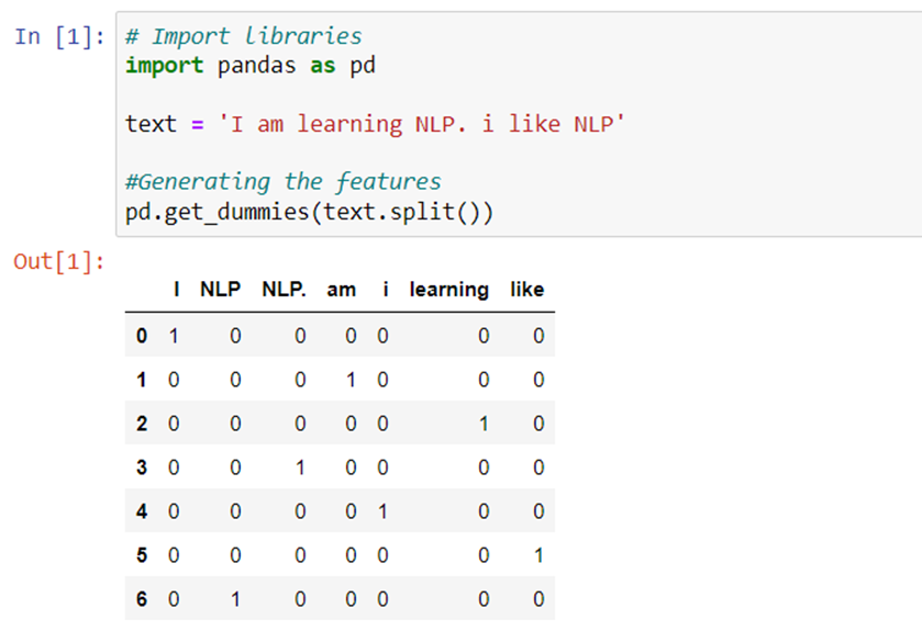
There are so many functions which we can use to generate One Hot encoding. We will take one function and discuss it in depth.
Converting Text to Features Using Count Vectorizing
This approach has a disadvantage. It doesn’t take the frequency of the word occurring into consideration. However, there’s a chance of missing the information if it isn’t included in the analysis, If a particular word is appearing multiple times. A count vectorizer will solve that problem. In this section, we will see the other method of converting text to feature, which is a count vectorizer.
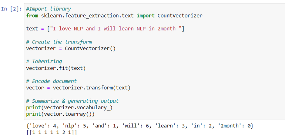
How it works
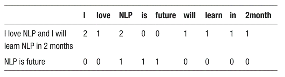
Count vectorizer is nearly analogous to One Hot encoding. The only difference is rather of checking whether the particular word is present or not, it’ll count the words that are present in the document. Observe the below illustration. The words “I” and “NLP” occur twice in the first document.
Generating N-grams
If you observe the above methods, each word is considered as a feature. There is a drawback to this method. It does not consider the previous and the next words, to see if that would give a proper and complete meaning to the words. For example: consider the word “not bad.” If this is split into individual words, then it will lose out on conveying “good” – which is what this word actually means. As we saw, we might lose potential information or insight because lot of words make sense once they are put together. This problem can be solved by N-grams. N-grams are the fusion of multiple letters or multiple words. They are formed in such a way that even the previous and next words are captured.
- Unigrams are the unique words present in the sentence.
- Bigram is the combination of 2 words.
- Trigram is 3 words and so on.
For example,
“I am learning NLP”
Unigrams: “I”, “am”, “learning”, “NLP”
Bigrams: “I am”, “am learning”, “learning NLP”
Trigrams: “I am learning”, “am learning NLP”
Generating N-grams using TextBlob

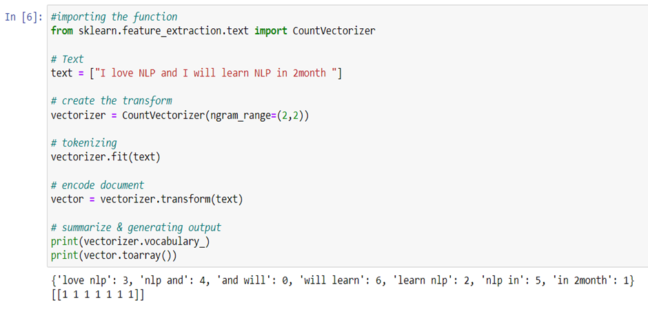
Bigram-based features for a document
Just like in the last recipe, we will use count vectorizer to generate features. Using the same function, let us generate bigram features and see what the output looks like.
Hash Vectorizing
A count vectorizer and co-occurrence matrix have one limitation though. In these methods, the vocabulary can become very large and cause memory/computation issues. One of the ways to solve this problem is a Hash Vectorizer.
Generate hash vectorizer matrix
Let’s create the Hashing Vectorizer of a vector size of 10.
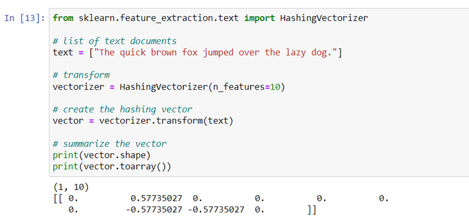
It created vector of size 10 and now this can be used for any supervised/unsupervised tasks.
Converting Text to Features Using TF-IDF
Again, in the above-mentioned text-to-feature methods, there are few drawbacks, hence the introduction of TF-IDF. Below are the disadvantages of the above methods.
- Let’s say a particular word is appearing in all the documents of the corpus, then it will achieve higher importance in our previous methods. That’s bad for our analysis.
- The whole idea of having TF-IDF is to reflect on how important a word is to a document in a collection, and hence normalizing words appeared frequently in all the documents.
Term frequency (TF)
Term frequency is simply the ratio of the count of a word present in a sentence, to the length of the sentence. TF is basically capturing the importance of the word irrespective of the length of the document. For example, a word with the frequency of 3 with the length of sentence being 10 is not the same as when the word length of sentence is 100 words. It should get more importance in the first scenario; that is what TF does.
Inverse Document Frequency (IDF)
IDF of each word is the log of the ratio of the total number of rows to the number of rows in a particular document in which that word is present.
IDF = log(N/n),
where N is the total number of rows and n is the number of rows in which the word was present. IDF will measure the rareness of a term. Words like “a,” and “the” show up in all the documents of the corpus, but rare words will not be there.
In all the documents. So, if a word is appearing in almost all documents, then that word is of no use to us since it is not helping to classify or in information retrieval. IDF will nullify this problem. TF-IDF is the simple product of TF and IDF so that both of the drawbacks are addressed, which makes predictions and information retrieval relevant.
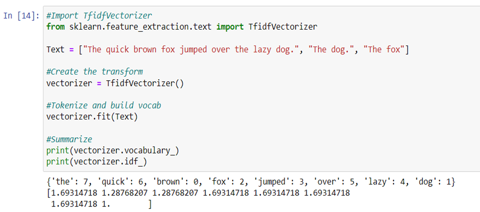
If you observe, “the” is appearing in all the 3 documents and it does not add much value, and hence the vector value is 1, which is less than all the other vector representations of the tokens. All these methods or techniques we have looked into so far are based on frequency and hence called frequency-based embeddings or features.
Implementing word embedding
This section assumes that you have a working knowledge of how a neural network works and the mechanisms by which weights in the neural network are updated. If new to a Neural Network (NN), it is suggested that you go through Chapter 6 to gain a basic understanding of how NN works.
Even though all previous methods solve most of the problems, once we get into more complicated problems where we want to capture the semantic relation between the words, these methods fail to perform.
Below are the challenges:
- All these techniques fail to capture the context and meaning of the words. All the methods discussed so far basically depend on the appearance or frequency of the words. But we need to look at how to capture the context or semantic relations: that is, how frequently the words are appearing close by.
a. I am eating an apple.
b. I am using apple.
If you observe the above example, Apple gives different meanings when it is used with different (close by) adjacent words, eating and using.
- For a problem like a document classification (book classification in the library), a document is really huge and there are a humongous number of tokens generated. In these scenarios, your number of features can get out of control (wherein) thus hampering the accuracy and performance.
A machine/algorithm can match two documents/texts and say whether they are same or not. But how do we make machines tell you about cricket or Virat Kohli when you search for MS Dhoni? How do you make a machine understand that “Apple” in “Apple is a tasty fruit” is a fruit that can be eaten and not a company? The answer to the above questions lies in creating a representation for words that capture their meanings, semantic relationships, and the different types of contexts they are used in. The above challenges are addressed by Word Embeddings. Word embedding is the feature learning technique where words from the vocabulary are mapped to vectors of real numbers capturing the contextual hierarchy. If you observe the below table, every word is represented with 4 numbers called vectors. Using the word embeddings technique, we are going to derive those vectors for each and every word so that we can use it in future analysis. In the below example, the dimension is 4. But we usually use a dimension greater than 100.
Word embeddings are prediction based, and they use shallow neural networks to train the model that will lead to learning the weight and using them as a vector representation.
word2vec: word2vec is the deep learning Google framework to train word embeddings. It will use all the words of the whole corpus and predict the nearby words. It will create a vector for all the words present in the corpus in a way so that the context is captured. It also outperforms any other methodologies in the space of word similarity and word analogies.
There are mainly 2 types in word2vec.
- Skip-Gram
- Continuous Bag of Words (CBOW)
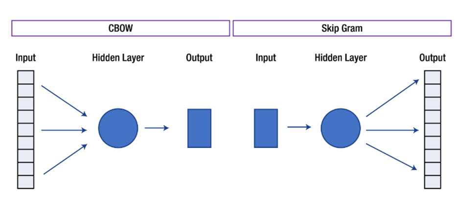
How It Works
The above figure shows the architecture of the CBOW and skip-gram algorithms used to build word embeddings. Let us see how these models work in detail.
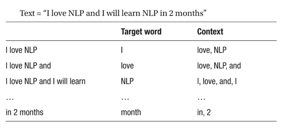
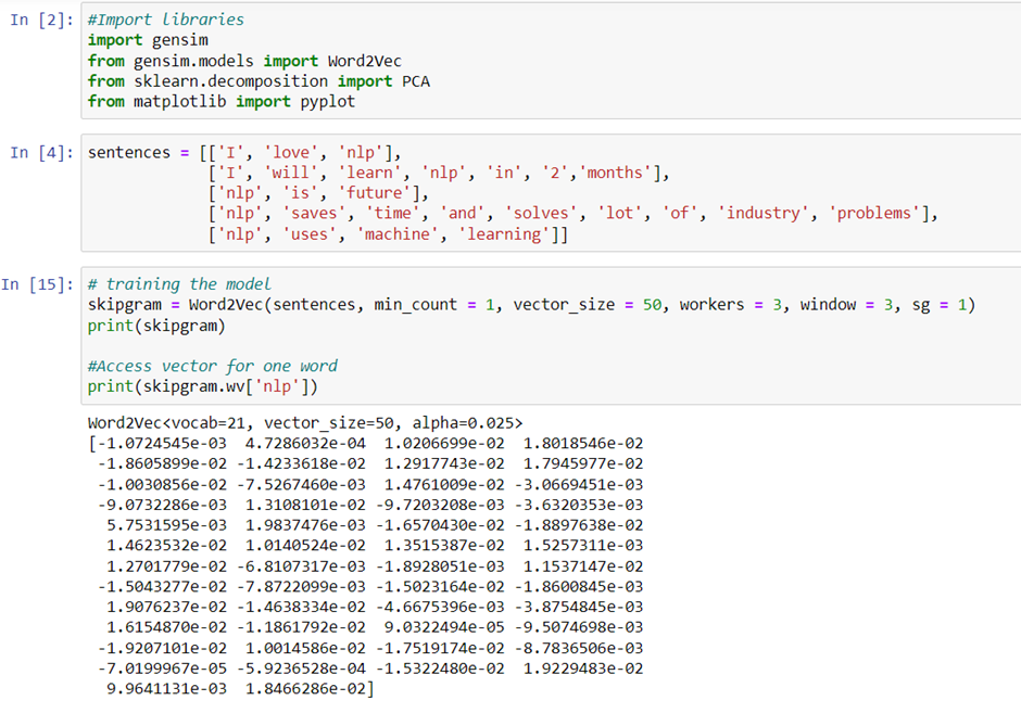
Skip-Gram
The skip-gram model (Mikolov et al., 2013)’is used to predict the probabilities of a word given the context of word or words. Let us take a small sentence and understand how it actually works. Each sentence will generate a target word and context, which are the words nearby. The number of words to be considered around the target variable is called the window size. The table below shows all the possible target and context variables for window size 2. Window size needs to be selected based on data and the resources at your disposal. The larger the window size, the higher the computing power.
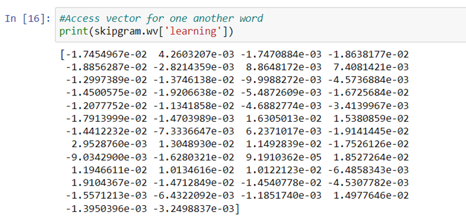
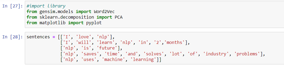
Since it takes a lot of text and computing power, let us go ahead and take sample data and build a skip-gram model.
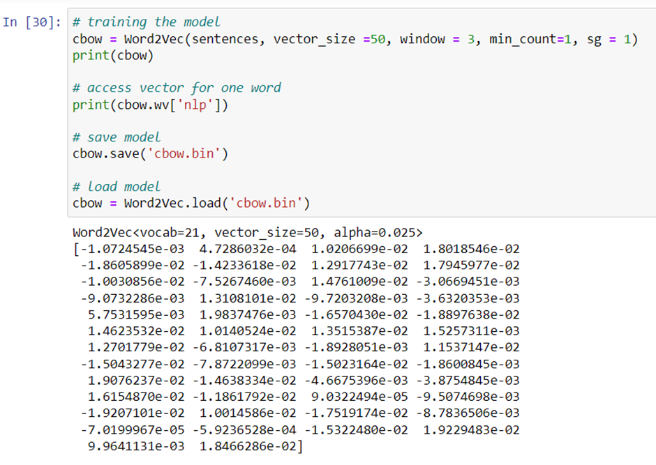
Continuous Bag of Words (CBOW)
Now let’s see how to build CBOW model.
Implementing fastText
fastText is another deep learning framework developed by Facebook to capture context and meaning.
fastText is the improvised version of word2vec. word2vec basically considers words to build the representation. But fastText takes each character while computing the representation of the word.
Let us see how to build a fastText word embedding.
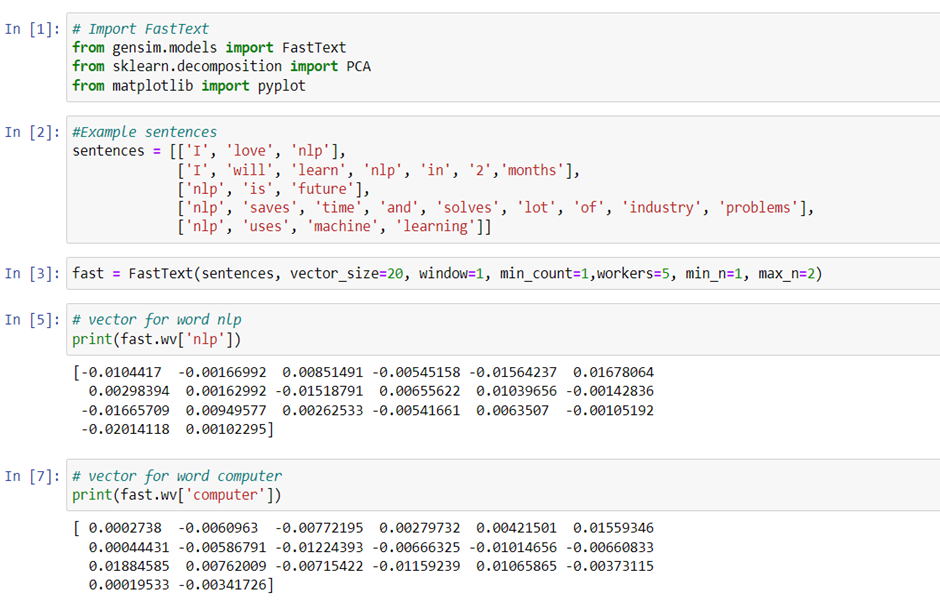
This is the advantage of using fastText. If any word not present in training of word2vec we would not get a vector for that. But since fastText is building on character level, even for the word that was not there in training, it will provide results. You can see the vector for the word “computer,” but it’s not present in the input data.

Nice article