We begin this chapter by examining a number of of the foremost image process algorithmic rule, then march on to machine learning implementation in image processing. The chapter at a look is as follows:
- Feature mapping using the scale-invariant feature transform (SIFT) algorithmic rule
Feature Mapping using the SIFT algorithmic rule Suppose we’ve 2 pictures. One image is of a bench in an exceedingly park. The second image is of the complete park, that additionally includes the bench. currently suppose we would like to put in writing code that helps us realize the bench within the park image.
You may assume this is often a simple task, however let me add some complexness. What if the image of the bench could be a zoomed image? Or what if it’s rotated? Or both? however square measure you attending to touch upon it now? the solution lies within the scale-invariant feature transform, or SIFT algorithmic rule. because the name recommend, it’s scale invariant, which suggests that despite what quantity we tend to pore on (or out of) the image, we are able to still realize similarities.
Another feature of this algorithmic rule is that it’s rotation invariant. regardless of degree of rotation, it still performs well. the sole issue with this algorithmic rule is that it’s proprietary, which suggests that for tutorial purposes it’s smart, except for industrial purpose there is also heap of legal problems involved with using it. However, this won’t stop us from learning and applying this algorithmic rule for currently. We initial should perceive the fundamentals of the algorithmic rule. Then we are able to apply it to finding similarities between 2 pictures using Python and so we’ll consider the code line by line.
Let’s consider the options of the image that the SIFT algorithmic rule tries to factor in throughout processing:
- Scale (zoomed-in or zoomed-out image)
- Rotation
- Illumination
- Perspective
As you’ll be able to see, not solely square measure scale and rotation accommodated, the SIFT algorithmic rule additionally takes care of the illumination gift within the image and also the perspective from that we tend to square measure trying. however however will it do all of this? Let’s take a glance at the in small stages method of using the SIFT algorithm:
- Realize and constructing an area to make sure scale invariance
- Realize the distinction between the gaussians
- Realize the details gift within the image
- Take away the unimportant points to create economical Comparisons
- Give orientation to the details found in step 3
- Identifying the key options uniquely.
Step 1: area Construction
In the start, we tend to take the first image and perform Gaussian blurring, in order that we are able to take away a number of the unimportant points and also the additional noise present within the image. once this is often done, we tend to size the image and repeat the method. There square measure varied factors on that resizing and blurring rely, however we tend to won’t go in the mathematical details here.
Step 2: distinction between the Gaussians
In the second step, we tend to take the pictures from step one and realize the distinction between their values. This makes the image scale invariant.
Step 3: Important points
details During the third step, we tend to establish details (also known as key points). The distinction between the gaussians image that we tend to found in step three is employed to see the native maxima and minima. we tend to take every constituent and so check its neighbors. The constituent is marked as a key purpose if it’s greatest (maximum) or least (minimum) among all its neighbors. ensuing step is to search out subpixel maxima and/or minima. we discover subpixels employing a mathematical conception known as the Taylor growth. once the subpixels square measure found, we tend to then try and realize the maxima and minima once more, using an equivalent method. Also, to solely take corners and take into account them as key points, we tend to use a mathematical conception known as the Hessian boot matrix. Corners square measure perpetually thought-about the simplest key points.
Step 4: Unimportant Key Points
In this step we first determine a threshold value. In the key points-generated image, and the subpixels image, we check the pixel intensity with the threshold value. If it is less than the threshold value, we consider it an unimportant key point and reject it.
Step 5: Orientation of Key Points
We find the direction of gradient and also the magnitude for every key purpose and its neighbors, then we glance at the foremost current orientation round the key purpose and assign an equivalent thereto. we tend to use histograms to search out these orientations and to induce the ultimate one.
Step 6: Key features
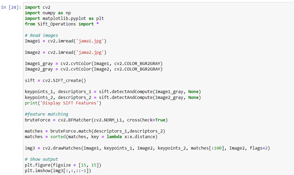
to make the key points distinctive, we tend to extract key options from them. Also, we tend to check that that whereas scrutiny these key points with the second image, they ought to not look precisely similar, however nearly similar. Now that we all know the fundamentals of the algorithmic rule, let’s consider the code to that algorithmic rule is applied to a try of pictures.


thanks for sharing information