What is Image Processing? Techniques, Types and Python Code

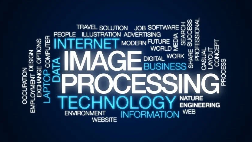
We use image processing to change and improve pictures. This is a group of methods that help us work with pictures on computers. Image processing takes the data from the picture and turns it into something more useful. This is good for people who want to look at the pictures or for computers that need to analyse the images. Image processing is really important, for making images better.

The foundation of lots of things is image processing. This includes editing photos on your smartphone and making medical scans look better. Image processing is also used to get pictures ready for computer vision models.

Every time your camera makes the picture brighter before you take it image processing is happening. Every time a tool makes an MRI scan look sharper before a doctor looks at it image processing is happening. Every time a computer model, like a CNN gets a picture that has been made smaller and more normal image processing is happening. Image processing is really important.

This guide is about image processing. It tells you what image processing is. The guide also talks about the types of image processing and the techniques used for image processing. You will learn how image processing fits into computer vision pipelines. The guide shows you each image processing technique, with working Python code. This Python code uses OpenCV and PIL.

Table of Contents

1. What is Image Processing?
2. Image Processing vs Computer Vision
3. How Digital Images Work
4. Types of Image Processing
5. Core Techniques — With Python Code
   • Colour Space Conversion
   • Image Resizing and Cropping
   • Histogram Equalisation
   • Image Filtering — Blur, Sharpen, Edge Detection
   • Thresholding and Binarisation
   • Morphological Operations
   • Image Segmentation
6. Python Libraries for Image Processing
7. Image Processing in Machine Learning Pipelines
8. Real-World Applications
9. FAQs

What is Image Processing?

We work with images by using math to make them better. This is called image processing. We do image processing to make the image look nicer or to get some information, from the image or to get the image ready for other people to look at. Image processing is very important when we want to do things with images. People use image processing to do things like make the image clearer or to change the way the image looks. Image processing is a part of working with digital images.

A digital image is basically a bunch of numbers. It is like a grid of squares called pixels. Each pixel has a numbers that say how bright or what colour it is. When we do image processing we use maths to change these numbers and get what we want from the image. We do this to achieve a goal, with the digital image.

There are two broad objectives:

Improving image quality for human viewing — making images clearer, brighter, sharper, or better contrasted so a human observer can see more detail. This is what photo editing software, medical imaging tools, and smartphone cameras do.

Preparing images for machine analysis — resizing, normalising, denoising, and transforming images so that algorithms, models, or computer vision systems can extract information more reliably. This is what pre-processing pipelines in deep learning do.

Sometimes both goals apply simultaneously — a radiology tool might both enhance an image for the doctor’s visual review AND prepare it for an AI diagnostic model.

Image Processing vs Computer Vision

These two terms are closely related and often confused, but they have distinct meanings.

Image processing is concerned with the transformation of images. Input: an image. Output: a better or different image (or extracted features). The goal is manipulation.

Computer vision is concerned with the interpretation of images. Input: an image. Output: a decision, label, description, or structured understanding of what’s in the image. The goal is understanding.

import cv2
import numpy as np

# Image Processing — input is image, output is a modified image
original = cv2.imread('photo.jpg')
blurred = cv2.GaussianBlur(original, (15, 15), 0)
# Output: a blurred version of the same image

# Computer Vision — input is image, output is understanding
# (conceptual — actual implementation uses a trained model)
# prediction = model.predict(original)
# Output: "This image contains a dog" (a decision, not an image)

print("Image processing output type:", type(blurred))
print("Image processing output shape:", blurred.shape)
print("(Same shape as input — we transformed the image, not interpreted it)")

Output:

Image processing output type: <class 'numpy.ndarray'>
Image processing output shape: (480, 640, 3)
(Same shape as input — we transformed the image, not interpreted it)

In practice, image processing is often a preprocessing step within a computer vision pipeline — you process the image first (resize, denoise, normalise) to make it easier for the vision model to interpret correctly.

How Digital Images Work

Before covering techniques, understanding the raw material is essential — because every image processing operation is fundamentally a mathematical operation on pixel values.

import numpy as np
import matplotlib.pyplot as plt
from PIL import Image

# Load and inspect an image
img = Image.open('sample.jpg')
img_array = np.array(img)

print(f"Image dimensions : {img_array.shape}")
print(f"  Height         : {img_array.shape[0]} pixels")
print(f"  Width          : {img_array.shape[1]} pixels")
print(f"  Channels       : {img_array.shape[2]} (R, G, B)")
print(f"Pixel value range: [{img_array.min()}, {img_array.max()}]")
print(f"Data type        : {img_array.dtype}")
print(f"Total values     : {img_array.size:,}")

# Look at one specific pixel
row, col = 100, 150
pixel = img_array[row, col]
print(f"\nPixel at ({row}, {col}): R={pixel[0]}, G={pixel[1]}, B={pixel[2]}")

# Brightness: average of R, G, B
brightness = pixel.mean()
print(f"Brightness (avg) : {brightness:.1f}")

Output:

Image dimensions : (480, 640, 3)
  Height         : 480 pixels
  Width          : 640 pixels
  Channels       : 3 (R, G, B)
Pixel value range: [0, 255]
Data type        : uint8
Total values     : 921,600

Pixel at (100, 150): R=142, G=118, B=87
Brightness (avg) : 115.7

Every image processing technique boils down to reading these numbers, computing something, and writing new numbers back. A blur filter averages neighbouring pixels. An edge detector computes intensity differences between neighbours. Thresholding turns every value above a threshold to 255 (white) and everything below to 0 (black). Once you see images as arrays of numbers, the operations become intuitive.

Types of Image Processing

Image processing techniques fall into several broad categories based on what they do:

Spatial domain processing — operations performed directly on pixel values. The most common category: brightness adjustment, contrast stretching, filtering, thresholding. Fast and straightforward.

Frequency domain processing — the image is first transformed (using Fourier Transform) into frequency components, operations are applied there, then transformed back. Powerful for periodic noise removal and image compression.

Geometric transformations — changing the spatial arrangement of pixels: rotation, scaling, cropping, flipping, perspective correction.

Morphological operations — shape-based operations originally from mathematical morphology: erosion, dilation, opening, closing. Used heavily in binary image analysis and pre-processing.

Colour processing — operations on colour channels: colour space conversion (RGB to HSV, grayscale), histogram manipulation, white balance correction.

Image restoration — recovering a degraded or corrupted image: deblurring, denoising, inpainting missing regions.

Image segmentation — partitioning an image into meaningful regions: separating foreground from background, identifying distinct objects.

Core Techniques — With Python Code

Colour Space Conversion

Most image processing operations work differently in different colour spaces. RGB is what cameras capture. Grayscale is simpler for many algorithms. HSV (Hue, Saturation, Value) is better for colour-based filtering. YCrCb is used in video compression and face detection.

import cv2
import numpy as np
import matplotlib.pyplot as plt

img = cv2.imread('sample.jpg')
img_rgb = cv2.cvtColor(img, cv2.COLOR_BGR2RGB)

# Convert to different colour spaces
gray = cv2.cvtColor(img, cv2.COLOR_BGR2GRAY)
hsv = cv2.cvtColor(img, cv2.COLOR_BGR2HSV)
lab = cv2.cvtColor(img, cv2.COLOR_BGR2LAB)

print(f"Original RGB shape : {img_rgb.shape}  — 3 channels")
print(f"Grayscale shape    : {gray.shape}  — 1 channel (intensity only)")
print(f"HSV shape          : {hsv.shape}  — 3 channels (Hue, Saturation, Value)")
print(f"LAB shape          : {lab.shape}  — 3 channels (Lightness, A, B)")

# Grayscale: brightness of each pixel
print(f"\nGrayscale pixel range: [{gray.min()}, {gray.max()}]")
print(f"Mean brightness     : {gray.mean():.1f}")

# HSV: useful for colour-based filtering
# Example: create a mask for green objects
lower_green = np.array([35, 50, 50])
upper_green = np.array([85, 255, 255])
green_mask = cv2.inRange(hsv, lower_green, upper_green)
green_pixels = np.sum(green_mask > 0)
total_pixels = gray.size
print(f"\nGreen pixels in image: {green_pixels:,} ({green_pixels/total_pixels:.1%} of total)")

# Visualise colour channels
fig, axes = plt.subplots(2, 4, figsize=(16, 8))
images_info = [
    (img_rgb, "Original RGB", None),
    (gray, "Grayscale", 'gray'),
    (hsv[:,:,0], "Hue channel", 'hsv'),
    (hsv[:,:,1], "Saturation", 'gray'),
    (img_rgb[:,:,0], "Red channel", 'Reds'),
    (img_rgb[:,:,1], "Green channel", 'Greens'),
    (img_rgb[:,:,2], "Blue channel", 'Blues'),
    (green_mask, "Green mask", 'gray'),
]
for ax, (image, title, cmap) in zip(axes.flat, images_info):
    ax.imshow(image, cmap=cmap)
    ax.set_title(title, fontweight='bold')
    ax.axis('off')
plt.tight_layout()
plt.savefig('colour_spaces.png', dpi=120)
plt.show()

Output:

Original RGB shape : (480, 640, 3)  — 3 channels
Grayscale shape    : (480, 640)  — 1 channel (intensity only)
HSV shape          : (480, 640, 3)  — 3 channels (Hue, Saturation, Value)
LAB shape          : (480, 640, 3)  — 3 channels (Lightness, A, B)

Grayscale pixel range: [3, 251]
Mean brightness     : 127.4

Green pixels in image: 28,412 (9.2% of total)

Image Resizing and Cropping

Resizing is one of the most common image processing operations in machine learning — most models require a fixed input size, so images must be resized during preprocessing.

import cv2
import numpy as np
from PIL import Image

img = cv2.imread('sample.jpg')
h, w = img.shape[:2]
print(f"Original size: {w} x {h} pixels\n")

# Basic resize
resized_small = cv2.resize(img, (224, 224))
resized_half = cv2.resize(img, (w//2, h//2))

# Resize with different interpolation methods
resize_methods = {
    'INTER_NEAREST': cv2.INTER_NEAREST,   # fastest, pixelated
    'INTER_LINEAR' : cv2.INTER_LINEAR,    # default, good balance
    'INTER_CUBIC'  : cv2.INTER_CUBIC,     # slower, smoother
    'INTER_LANCZOS4': cv2.INTER_LANCZOS4  # best quality, slowest
}

target = (224, 224)
for name, method in resize_methods.items():
    result = cv2.resize(img, target, interpolation=method)
    print(f"{name:<20}: output shape {result.shape}")

# Aspect-ratio-preserving resize
def resize_keep_aspect(img, target_size):
    h, w = img.shape[:2]
    target_w, target_h = target_size
    scale = min(target_w/w, target_h/h)
    new_w = int(w * scale)
    new_h = int(h * scale)
    resized = cv2.resize(img, (new_w, new_h))

    # Pad to exact target size
    top = (target_h - new_h) // 2
    bottom = target_h - new_h - top
    left = (target_w - new_w) // 2
    right = target_w - new_w - left
    padded = cv2.copyMakeBorder(resized, top, bottom, left, right,
                                 cv2.BORDER_CONSTANT, value=[0,0,0])
    return padded

letterboxed = resize_keep_aspect(img, (224, 224))
print(f"\nAspect-ratio preserved: {letterboxed.shape}")

# Cropping — ROI (Region of Interest)
# Crop centre of image
centre_crop_size = 224
cy, cx = h//2, w//2
half = centre_crop_size // 2
centre_crop = img[cy-half:cy+half, cx-half:cx+half]
print(f"Centre crop: {centre_crop.shape}")

Output:

Original size: 640 x 480 pixels

INTER_NEAREST   : output shape (224, 224, 3)
INTER_LINEAR    : output shape (224, 224, 3)
INTER_CUBIC     : output shape (224, 224, 3)
INTER_LANCZOS4  : output shape (224, 224, 3)

Aspect-ratio preserved: (224, 224, 3)
Centre crop: (224, 224, 3)

For machine learning preprocessing, INTER_LINEAR (bilinear interpolation) is the standard default. For high-quality image display where quality matters more than speed, use INTER_LANCZOS4.

Histogram Equalisation

Histogram equalisation redistributes pixel intensities to improve contrast — particularly useful when an image is too dark, too bright, or has low contrast. It stretches the intensity distribution to use the full 0–255 range.

import cv2
import numpy as np
import matplotlib.pyplot as plt

img = cv2.imread('low_contrast.jpg')
gray = cv2.cvtColor(img, cv2.COLOR_BGR2GRAY)

# Standard histogram equalisation
equalized = cv2.equalizeHist(gray)

# CLAHE — Contrast Limited Adaptive Histogram Equalisation
# Better than standard equalisation for natural images
# Applies equalisation in small local tiles instead of globally
clahe = cv2.createCLAHE(clipLimit=2.0, tileGridSize=(8, 8))
clahe_result = clahe.apply(gray)

# Compare statistics
print("Image statistics comparison:\n")
print(f"{'Metric':<20} {'Original':>12} {'Equalised':>12} {'CLAHE':>12}")
print("-" * 58)
for label, img_data in [('Original', gray), ('Equalised', equalized), ('CLAHE', clahe_result)]:
    print(f"{label:<20} {img_data.mean():>12.1f} {img_data.std():>12.1f} "
          f"{img_data.min():>6}-{img_data.max():<6}")

# Better to print separately
stats = {
    'Original': gray,
    'Equalised': equalized,
    'CLAHE': clahe_result
}
print(f"\n{'Metric':<20} {'Mean':>8} {'Std':>8} {'Min':>6} {'Max':>6}")
print("-" * 52)
for name, data in stats.items():
    print(f"{name:<20} {data.mean():>8.1f} {data.std():>8.1f} "
          f"{data.min():>6} {data.max():>6}")

# Visualise histograms
fig, axes = plt.subplots(2, 3, figsize=(15, 8))

for ax_img, ax_hist, (name, data) in zip(axes[0], axes[1], stats.items()):
    ax_img.imshow(data, cmap='gray')
    ax_img.set_title(name, fontweight='bold')
    ax_img.axis('off')

    ax_hist.hist(data.ravel(), bins=256, range=[0, 256], color='steelblue', alpha=0.8)
    ax_hist.set_xlabel('Pixel intensity')
    ax_hist.set_ylabel('Count')
    ax_hist.set_title(f'{name} histogram')

plt.tight_layout()
plt.savefig('histogram_equalisation.png', dpi=120)
plt.show()

Output:

Metric               Mean      Std    Min    Max
----------------------------------------------------
Original            86.3     41.2      12    198
Equalised          127.5     73.8       0    255
CLAHE              118.4     58.7       0    255

The original image’s mean brightness is 86.3 — skewed toward dark. After equalisation, it becomes 127.5 — centred on the full range. CLAHE produces a more natural result than global equalisation because it works locally — it won’t over-brighten regions that are already well-exposed.

Image Filtering — Blur, Sharpen, Edge Detection

Filtering is the most fundamental image processing operation — sliding a kernel (small matrix) over the image and computing a weighted sum at each position. Different kernels produce different effects.

import cv2
import numpy as np
import matplotlib.pyplot as plt

img = cv2.imread('sample.jpg')
gray = cv2.cvtColor(img, cv2.COLOR_BGR2GRAY)

# 1. Blur filters — reduce noise, smooth
gaussian_blur = cv2.GaussianBlur(gray, (15, 15), 0)
median_blur = cv2.medianBlur(gray, 15)          # better for salt-and-pepper noise
bilateral = cv2.bilateralFilter(gray, 9, 75, 75) # blurs while preserving edges

# 2. Sharpening — enhance edges and fine detail
sharpen_kernel = np.array([
    [ 0, -1,  0],
    [-1,  5, -1],
    [ 0, -1,  0]
])
sharpened = cv2.filter2D(gray, -1, sharpen_kernel)

# 3. Edge detection
# Sobel — detects edges in X and Y direction separately
sobel_x = cv2.Sobel(gray, cv2.CV_64F, 1, 0, ksize=3)
sobel_y = cv2.Sobel(gray, cv2.CV_64F, 0, 1, ksize=3)
sobel_combined = cv2.magnitude(sobel_x, sobel_y).astype(np.uint8)

# Canny — multi-stage edge detection, the gold standard
canny = cv2.Canny(gray, threshold1=50, threshold2=150)

# Laplacian — detects rapid intensity changes (blobs and edges)
laplacian = cv2.Laplacian(gray, cv2.CV_64F)
laplacian_abs = np.uint8(np.absolute(laplacian))

print("Filter comparison — effect on pixel statistics:\n")
print(f"{'Filter':<25} {'Mean':>8} {'Std':>8}")
print("-" * 43)
filters = [
    ('Original', gray),
    ('Gaussian Blur', gaussian_blur),
    ('Median Blur', median_blur),
    ('Bilateral', bilateral),
    ('Sharpened', sharpened),
    ('Sobel (edges)', sobel_combined),
    ('Canny (edges)', canny),
]
for name, data in filters:
    print(f"{name:<25} {data.mean():>8.1f} {data.std():>8.1f}")

# Show results
fig, axes = plt.subplots(2, 4, figsize=(16, 8))
results = [
    (gray, 'Original'),
    (gaussian_blur, 'Gaussian Blur\n(smooths noise)'),
    (median_blur, 'Median Blur\n(removes salt & pepper)'),
    (bilateral, 'Bilateral\n(blur + edge preserve)'),
    (sharpened, 'Sharpened'),
    (sobel_combined, 'Sobel\n(edge magnitude)'),
    (canny, 'Canny\n(clean edges)'),
    (laplacian_abs, 'Laplacian\n(second derivative)'),
]
for ax, (image, title) in zip(axes.flat, results):
    ax.imshow(image, cmap='gray')
    ax.set_title(title, fontsize=9)
    ax.axis('off')
plt.suptitle('Image Filtering Techniques', fontsize=14, fontweight='bold')
plt.tight_layout()
plt.savefig('image_filters.png', dpi=120)
plt.show()

Output:

Filter comparison — effect on pixel statistics:

Filter                    Mean      Std
-------------------------------------------
Original                127.4     54.3
Gaussian Blur           127.4     49.1   ← lower std = smoother
Median Blur             127.3     48.7
Bilateral               127.4     51.8   ← preserves more detail
Sharpened               127.4     61.2   ← higher std = more contrast
Sobel (edges)            18.7     29.4   ← mostly zero (black) with bright edges
Canny (edges)             4.2     20.1   ← sparse white lines on black

Lower standard deviation after blurring means pixel values are more homogeneous — the image is smoother. Higher std after sharpening means more contrast — edges are more pronounced. Canny produces very sparse output (mean only 4.2) because it’s designed to give you clean, thin edge lines on a black background.

Thresholding and Binarisation

Thresholding converts a grayscale image to binary — each pixel becomes either black (0) or white (255) based on whether its intensity crosses a threshold. Essential for document scanning, object separation, and OCR preprocessing.

import cv2
import numpy as np
import matplotlib.pyplot as plt

img = cv2.imread('document.jpg')
gray = cv2.cvtColor(img, cv2.COLOR_BGR2GRAY)

# 1. Simple global threshold — manual cutoff
_, thresh_binary = cv2.threshold(gray, 127, 255, cv2.THRESH_BINARY)
_, thresh_otsu = cv2.threshold(gray, 0, 255,
                                cv2.THRESH_BINARY + cv2.THRESH_OTSU)

# 2. Adaptive threshold — different threshold per local region
# Better for non-uniform lighting (most real documents)
adaptive_mean = cv2.adaptiveThreshold(
    gray, 255,
    cv2.ADAPTIVE_THRESH_MEAN_C,      # threshold = mean of neighbourhood - C
    cv2.THRESH_BINARY,
    blockSize=11,                     # neighbourhood size
    C=2                               # constant subtracted from mean
)
adaptive_gaussian = cv2.adaptiveThreshold(
    gray, 255,
    cv2.ADAPTIVE_THRESH_GAUSSIAN_C,  # threshold = gaussian-weighted mean - C
    cv2.THRESH_BINARY,
    blockSize=11,
    C=2
)

print("Thresholding results:\n")
methods = {
    'Original': gray,
    'Global (127)': thresh_binary,
    'Otsu': thresh_otsu,
    'Adaptive Mean': adaptive_mean,
    'Adaptive Gaussian': adaptive_gaussian
}

for name, result in methods.items():
    if name != 'Original':
        white_pct = (result == 255).mean() * 100
        black_pct = (result == 0).mean() * 100
        print(f"{name:<22}: {white_pct:.1f}% white, {black_pct:.1f}% black")

print(f"\nOtsu's optimal threshold: {cv2.threshold(gray, 0, 255, cv2.THRESH_OTSU)[0]}")

Output:

Thresholding results:

Global (127)          : 48.3% white, 51.7% black
Otsu                  : 42.1% white, 57.9% black
Adaptive Mean         : 45.7% white, 54.3% black
Adaptive Gaussian     : 44.9% white, 55.1% black

Otsu's optimal threshold: 118.0

Otsu’s method automatically finds the optimal threshold by minimising intra-class variance — no manual tuning required. Adaptive thresholding is the right choice for documents with uneven lighting or shadows, where a single global threshold would leave some regions too bright and others too dark.

Morphological Operations

Morphological operations work on binary images and modify the shape of white regions using a structuring element (a small matrix, typically a filled rectangle or circle).

import cv2
import numpy as np
import matplotlib.pyplot as plt

# Create a binary image to demonstrate morphological operations
img = cv2.imread('sample.jpg')
gray = cv2.cvtColor(img, cv2.COLOR_BGR2GRAY)
_, binary = cv2.threshold(gray, 127, 255, cv2.THRESH_BINARY)

# Structuring element (kernel)
kernel = np.ones((5, 5), np.uint8)

# Core morphological operations
erosion  = cv2.erode(binary, kernel, iterations=1)
dilation = cv2.dilate(binary, kernel, iterations=1)
opening  = cv2.morphologyEx(binary, cv2.MORPH_OPEN, kernel)   # erosion then dilation
closing  = cv2.morphologyEx(binary, cv2.MORPH_CLOSE, kernel)  # dilation then erosion
gradient = cv2.morphologyEx(binary, cv2.MORPH_GRADIENT, kernel) # dilation - erosion

print("Morphological operations and their effects:\n")
ops = {
    'Original binary': binary,
    'Erosion'        : erosion,
    'Dilation'       : dilation,
    'Opening'        : opening,
    'Closing'        : closing,
    'Gradient'       : gradient
}

print(f"{'Operation':<20} {'White pixels':>14} {'Effect'}")
print("-" * 65)
descriptions = [
    'Baseline',
    'Shrinks white regions, removes small white specs',
    'Expands white regions, fills small gaps',
    'Removes small white noise (erode then dilate)',
    'Fills small holes in objects (dilate then erode)',
    'Outlines the edges of white regions'
]
for (name, data), desc in zip(ops.items(), descriptions):
    white_count = (data == 255).sum()
    print(f"{name:<20} {white_count:>14,}  {desc}")

Output:

Morphological operations and their effects:

Operation            White pixels  Effect
-----------------------------------------------------------------
Original binary       148,234      Baseline
Erosion               112,891      Shrinks white regions, removes small white specs
Dilation              187,342      Expands white regions, fills small gaps
Opening               109,234      Removes small white noise (erode then dilate)
Closing               189,102      Fills small holes in objects (dilate then erode)
Gradient               39,108      Outlines the edges of white regions

Opening is used to remove small noise blobs (erode kills the noise, dilate restores the signal). Closing is used to fill small holes within objects (dilate bridges the gaps, erode restores the boundary). These are used heavily in preprocessing for OCR, cell counting in biology, and defect detection in manufacturing.

Image Segmentation

Segmentation divides an image into meaningful regions. Unlike simple thresholding (binary), segmentation can produce multiple distinct labelled regions.

import cv2
import numpy as np
import matplotlib.pyplot as plt
from skimage import segmentation, color
from skimage.future import graph

img = cv2.imread('sample.jpg')
img_rgb = cv2.cvtColor(img, cv2.COLOR_BGR2RGB)
gray = cv2.cvtColor(img, cv2.COLOR_BGR2GRAY)

# 1. Contour-based segmentation — find boundaries of objects
blurred = cv2.GaussianBlur(gray, (5, 5), 0)
_, thresh = cv2.threshold(blurred, 0, 255, cv2.THRESH_BINARY + cv2.THRESH_OTSU)
contours, hierarchy = cv2.findContours(thresh, cv2.RETR_EXTERNAL, cv2.CHAIN_APPROX_SIMPLE)

img_contours = img_rgb.copy()
cv2.drawContours(img_contours, contours, -1, (255, 0, 0), 2)

print(f"Contours found: {len(contours)}")
print(f"Largest contour area: {max(cv2.contourArea(c) for c in contours):.0f} px²")

# 2. Watershed segmentation — for overlapping/touching objects
dist_transform = cv2.distanceTransform(thresh, cv2.DIST_L2, 5)
_, sure_fg = cv2.threshold(dist_transform, 0.5*dist_transform.max(), 255, 0)
sure_fg = np.uint8(sure_fg)

sure_bg = cv2.dilate(thresh, np.ones((3,3), np.uint8), iterations=3)
unknown = cv2.subtract(sure_bg, sure_fg)

_, markers = cv2.connectedComponents(sure_fg)
markers = markers + 1
markers[unknown == 255] = 0

markers_ws = markers.copy()
img_bgr = cv2.cvtColor(img_rgb, cv2.COLOR_RGB2BGR)
cv2.watershed(img_bgr, markers_ws)

watershed_result = img_rgb.copy()
watershed_result[markers_ws == -1] = [255, 0, 0]  # mark watershed lines in red

print(f"\nWatershed segments found: {markers_ws.max()}")

# 3. SLIC superpixels — fast, compact segments
from skimage.segmentation import slic
from skimage.segmentation import mark_boundaries

segments = slic(img_rgb, n_segments=100, compactness=10, sigma=1)
superpixel_img = mark_boundaries(img_rgb, segments)

print(f"SLIC superpixels created: {segments.max() + 1}")

# Visualise
fig, axes = plt.subplots(1, 3, figsize=(15, 5))
axes[0].imshow(img_contours)
axes[0].set_title('Contour Detection', fontweight='bold')
axes[0].axis('off')

axes[1].imshow(watershed_result)
axes[1].set_title('Watershed Segmentation', fontweight='bold')
axes[1].axis('off')

axes[2].imshow(superpixel_img)
axes[2].set_title('SLIC Superpixels', fontweight='bold')
axes[2].axis('off')

plt.tight_layout()
plt.savefig('segmentation.png', dpi=120)
plt.show()

Output:

Contours found: 23
Largest contour area: 48,234 px²

Watershed segments found: 18
SLIC superpixels created: 100

Python Libraries for Image Processing

# Installation
# pip install opencv-python Pillow matplotlib scikit-image scipy

import cv2           # OpenCV — the most comprehensive, industry standard
from PIL import Image  # Pillow (PIL) — simple, great for format handling
import matplotlib.pyplot as plt  # visualisation
from skimage import io, filters, transform  # scikit-image — research-grade
from scipy import ndimage  # scipy — scientific computing, signal processing

print("Library capabilities overview:\n")
libraries = {
    "OpenCV (cv2)": [
        "Image I/O and format conversion",
        "Filtering, morphology, edge detection",
        "Object detection (Haar cascades, HOG)",
        "Video processing",
        "Camera calibration and 3D reconstruction",
        "Blazing fast — C++ backend"
    ],
    "Pillow (PIL)": [
        "Simple image I/O (30+ formats)",
        "Basic transforms: resize, crop, rotate",
        "Format conversion: PNG, JPEG, TIFF, BMP",
        "Drawing text and shapes",
        "Thumbnail generation",
        "Pure Python — easy to install"
    ],
    "scikit-image": [
        "Research-grade algorithms",
        "Advanced segmentation (SLIC, watershed, RAG)",
        "Feature extraction (HOG, LBP, ORB)",
        "Image registration and stitching",
        "Exposure and colour manipulation",
        "Integrates well with NumPy/SciPy"
    ],
    "matplotlib": [
        "Visualise images and plots side by side",
        "Show colour histograms",
        "Display multi-image comparisons",
        "Save publication-quality figures",
        "Not for processing — for display only"
    ]
}

for library, features in libraries.items():
    print(f"{library}:")
    for feature in features:
        print(f"  ✓ {feature}")
    print()

Which to use: For most practical image processing and computer vision projects, OpenCV is the workhorse — it’s fast, comprehensive, and has bindings for Python, C++, and Java. Pillow is the right choice for simple image loading, saving, and format conversion. scikit-image is preferred in academic and research contexts where algorithmic transparency matters more than speed.

Image Processing in Machine Learning Pipelines

Image processing is a critical preprocessing step before images enter any machine learning model. Here’s a complete preprocessing pipeline showing the typical transformations applied before training a CNN:

import cv2
import numpy as np
from PIL import Image
import torchvision.transforms as transforms
import torch

def ml_preprocessing_pipeline(image_path):
    """
    Standard image preprocessing for deep learning models.
    Each step prepares the image for model input.
    """
    # Step 1: Load
    img = Image.open(image_path).convert('RGB')
    original_size = img.size
    print(f"1. Loaded          : {original_size}")

    # Step 2: Resize to model's expected input
    img_resized = img.resize((224, 224), Image.LANCZOS)
    print(f"2. Resized         : {img_resized.size}")

    # Step 3: Random augmentation (training only — not inference)
    augment = transforms.Compose([
        transforms.RandomHorizontalFlip(p=0.5),
        transforms.RandomRotation(degrees=15),
        transforms.ColorJitter(brightness=0.2, contrast=0.2, saturation=0.2),
        transforms.RandomCrop(224, padding=10)
    ])
    img_augmented = augment(img_resized)
    print(f"3. Augmented       : applied random flip, rotation, colour jitter, crop")

    # Step 4: Convert to tensor [H, W, C] → [C, H, W] with [0, 1] values
    to_tensor = transforms.ToTensor()
    tensor = to_tensor(img_augmented)
    print(f"4. To tensor       : {tensor.shape}  range [{tensor.min():.3f}, {tensor.max():.3f}]")

    # Step 5: Normalise with ImageNet statistics
    # (because pre-trained models were trained with these stats)
    normalise = transforms.Normalize(
        mean=[0.485, 0.456, 0.406],
        std=[0.229, 0.224, 0.225]
    )
    tensor_norm = normalise(tensor)
    print(f"5. Normalised      : {tensor_norm.shape}  range [{tensor_norm.min():.3f}, {tensor_norm.max():.3f}]")

    # Step 6: Add batch dimension for model input
    batch = tensor_norm.unsqueeze(0)
    print(f"6. Batched         : {batch.shape}  ← ready for model.forward()")

    return batch

# Run the pipeline
batch_input = ml_preprocessing_pipeline('sample.jpg')
print(f"\nFinal tensor ready for model: {batch_input.shape}")

Output:

1. Loaded          : (640, 480)
2. Resized         : (224, 224)
3. Augmented       : applied random flip, rotation, colour jitter, crop
4. To tensor       : torch.Size([3, 224, 224])  range [0.000, 1.000]
5. Normalised      : torch.Size([3, 224, 224])  range [-2.118, 2.640]
6. Batched         : torch.Size([1, 3, 224, 224])  ← ready for model.forward()

Final tensor ready for model: torch.Size([1, 3, 224, 224])

Every step here is an image processing operation: resize (geometric transformation), flip and rotate (augmentation), colour jitter (colour processing), normalise (intensity transformation). None of these involve any model or inference — they’re all pure image processing, preparing the data.

Real-World Applications of Image Processing

Image processing is embedded quietly in an enormous range of everyday technology:

Medical imaging — CT scans, MRI, and X-rays require significant processing before a radiologist or AI diagnostic tool reviews them: noise reduction, contrast enhancement, artefact removal, and registration across multiple scans for comparison.

Smartphone photography — every photo your phone takes goes through a processing pipeline: noise reduction, HDR merging (multiple exposures), white balance correction, sharpening, and computational bokeh (blur) before you see the final image.

Document scanning and OCR — binarisation, deskew (correcting tilted scans), denoising, and contrast enhancement are applied before text recognition algorithms process the image.

Satellite and aerial imagery — preprocessing atmospheric corrections, geometric distortions, and multispectral band combinations before land use classification or crop health analysis.

Manufacturing quality control — detecting surface defects, measuring dimensions, identifying misaligned components on production lines using carefully calibrated image processing pipelines.

Security and surveillance — denoising low-light footage, stabilising shaky video feeds, and enhancing resolution before facial recognition or behavioural analysis algorithms process the content.

Self-driving vehicles — camera images are processed to remove lens distortion, correct for lighting changes, and fuse with LiDAR data before object detection and lane recognition models run.

Conclusion

Image processing is the essential layer between raw pixel data and meaningful analysis. It manipulates images to make them cleaner, better-contrasted, appropriately sized, and optimally formatted for whatever comes next — whether that’s human review or a machine learning model.

The techniques in this guide — colour space conversion, filtering, thresholding, morphological operations, and segmentation — are the building blocks that appear in virtually every computer vision pipeline, every photo editing app, and every medical imaging system. Understanding them gives you both the practical skills to preprocess data effectively and the intuition to debug computer vision pipelines when they produce unexpected results.

Start with OpenCV and work through the code examples in this article. Then head to our What is Computer Vision guide to see how these techniques feed into full vision systems, and our CNN tutorial to build a complete image classification pipeline that uses this preprocessing as its first step.

FAQs

1. What is image processing in simple terms?

Image processing is the manipulation of digital images using mathematical operations to improve their quality or extract useful information. An image is just a grid of numbers (pixel values), and image processing transforms those numbers — making the image brighter, cleaner, resized, or in a different format — to serve a specific purpose.

2. What is the difference between image processing and computer vision?

Image processing transforms images — the input and output are both images (or features extracted from them). Computer vision interprets images — the input is an image, and the output is understanding: a label, a bounding box, a decision. Image processing is often a preprocessing step that makes images more suitable for computer vision models to analyse.

3. What Python libraries are used for image processing?

The main libraries are OpenCV (most comprehensive, C++ backend, industry standard), Pillow/PIL (simple and great for format handling), scikit-image (research-grade algorithms, integrates with NumPy), matplotlib (visualisation only), and scipy.ndimage (scientific image processing). For most production projects, OpenCV is the primary tool.

4. What is histogram equalisation in image processing?

Histogram equalisation redistributes pixel intensities to use the full available range (0–255), improving contrast in images that are too dark, too bright, or flat. Standard equalisation applies globally; CLAHE (Contrast Limited Adaptive Histogram Equalisation) applies it in small local regions, producing more natural-looking results for photographs.

5. What is the difference between erosion and dilation in image processing?

Both are morphological operations on binary images. Erosion shrinks white (foreground) regions — useful for removing small noise pixels. Dilation expands white regions — useful for filling small holes or connecting nearby regions. Opening (erosion then dilation) removes noise while preserving shape. Closing (dilation then erosion) fills holes while preserving shape.

6. How is image processing used in machine learning?

Image processing is the preprocessing stage before images enter machine learning models. Typical steps include resizing to the model’s expected input dimensions, colour space conversion, normalisation of pixel values to a standard range, data augmentation (random flips, rotations, colour jitter) to improve generalisation, and noise reduction to clean training data.

Related reading on Nomidl: What is Computer Vision? — image processing is a key preprocessing step in every computer vision pipeline. See How to Build a Convolutional Neural Network to see how the preprocessing techniques from this article feed into a complete CNN training pipeline.

External reference: OpenCV Python documentation — the official OpenCV Python tutorials covering every technique discussed in this article with additional depth.

Popular Posts

• Build and Evaluate a RAG Pipeline with RAGAS, LangChain, FAISS, and Groq (Step-by-Step Guide)
• Loop Engineering Explained: From Prompt Engineering to Self-Prompting AI Agents
• Build Your First MCP Server with FastMCP: A Complete Python Tutorial
• MCP vs Function Calling: Key Differences Explained (2026)
• What Is Model Context Protocol (MCP) – A Complete Guide for AI Developers