Nomidl

Advance image processing using OpenCV

• Naveen
• June 18, 2022December 12, 2024
• 0

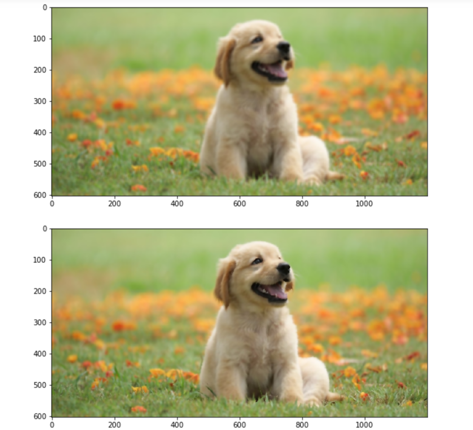
Blending two images

Suppose you have two images and you want to blend them so that features of both images are visible. We use image registration techniques to blend one image over the second one and determine whether there are any changes. Let’s look at the code.

Let’s look at some of the functions used in this code:

• Import cv2: The complete OpenCV library is present in the package cv2. So we need to import this package to use the classes and function stored in it.
  
• cv2.imread(): Similar to skimage.io.imread(), we have cv2.imread(), which is used to read the image from a particular destination.
  
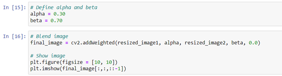
• cv2.addWeighted(): This function blends the two images. The alpha and beta parameters indicate the transparency in both images. There are a few formulas that help to determine the final blending. The last parameter is called gamma. Currently it has a value of zero. It’s just a scaler, which is added to the formulas, to transform the images more effectively. In general, gamma is zero.
  
• cv2.imshow(): Similar to skimage.io.imshow(), cv2.imshow() helps to display the image in  a new window.
  
• cv2.waitKey(): waitKey() is used so that the window displaying the output remains until we click close or pressed Escape, this function destroys all the windows that have been opened and saved in the memory.

Following pictures are the output of the previous code:

Changing Contrast and Brightness

To change contrast and brightness in image, we should have an understanding of what these two terms mean:

• Contrast: Contrast is the difference between maximum and minimum pixel intensity.
  
• Brightness: Brightness refers to the lightness or darkness of an image. To make an image brighter, we add a constant number to all the pixels present in it.

Let’s look at the code and the output, to see the difference between contrast and brightness.

In this code, we did not use any cv2 functions to change the brightness or contrast. We used the numpy library and a slicing concept to change the parameters. The first thing we did was define the parameters. We gave contrast a value of 3 and brightness a value of 2. The first for loop gave the image channels. Therefore, the first loop runs width a number of times, the second loop runs height a number of times, and the last loop runs the number of color channels a number of times. If the RGB image is there, then loop runs three times for the three channels.

np.clip() limits the value in a particular range. In the previous code, the range is 0 to 255, which is nothing but the pixel values for each channel. So, a formula is derived:

(Specific pixel value * Contrast) + Brightness.

Using the formula, we can change each and every pixel value, and np.clip() makes sure the output value doesn’t go beyond 0 to 255. Hence, the loops traverse through each and every pixel, for each and every channel, and does the transformation.

Here is the output images:

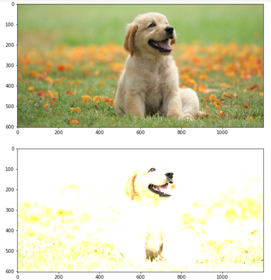
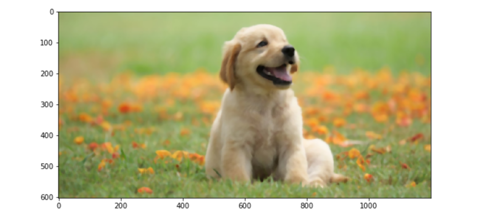
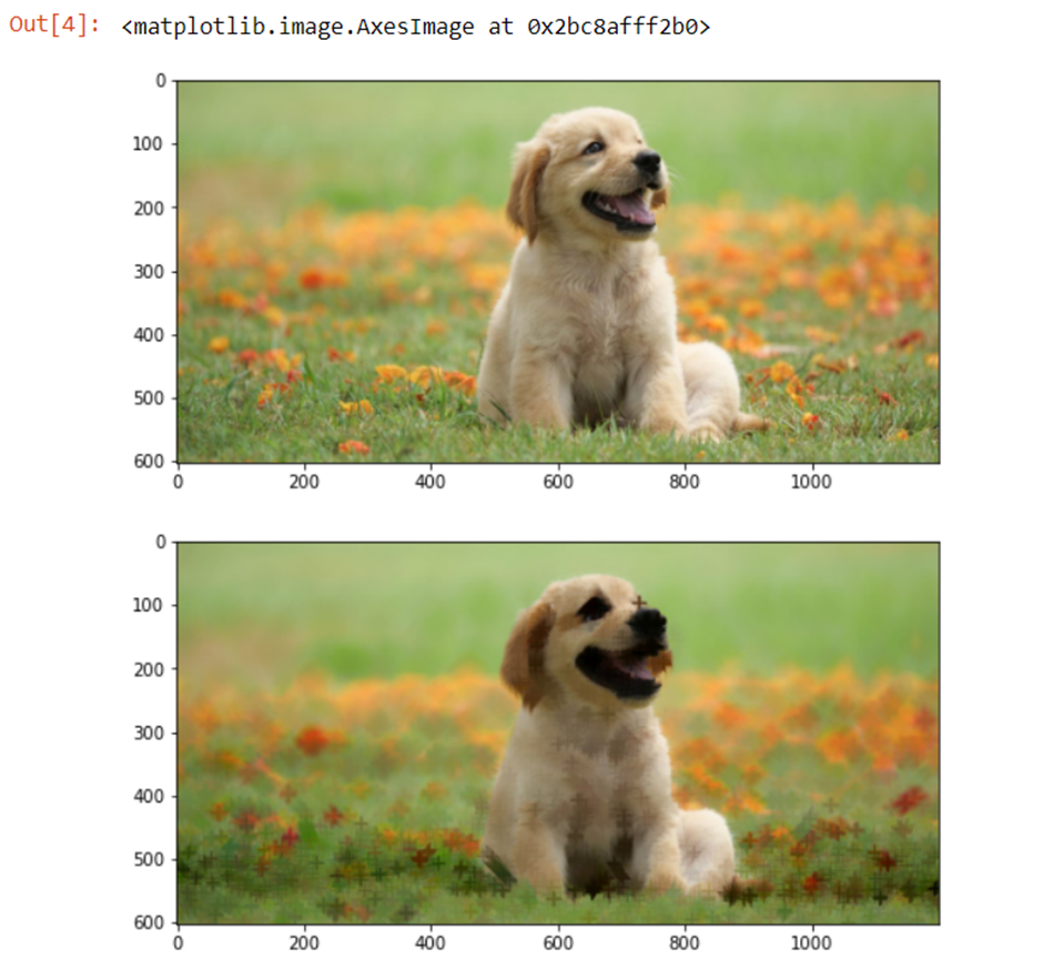
Smoothing images

In this section we take a look at three filters used to smooth images. These filters are as follow:

• The median filter (cv2.medianBlur)
  
• The gaussian filter (cv2.GaussianBlur)
  
• The bilateral filter (cv2.bilateralFilter)

Median Filter

The median filter is one of the most introductory image-smoothing filters. It’s nonlinear filter that removes black and white noise present ina n image by finding the median using neighboring pixels.

To smooth an image using the median filter, we look at the first 3 * 3 matrix, find the median of that matrix, then remove the central value by the median. Next, we move one step to the right and repeat this process until all the pixels have been covered. The final image is a smoothed image. If you want to preserve the edges of your image while blurring, the median filter is your stylish option.

Cv2.medianBlur is the function used to achieve median blur. It has two parameters:

1 – The image we want to smooth

2 – The kernel size, which should be odd. Therefore, a value of 9 means 9 x 9 matrix.

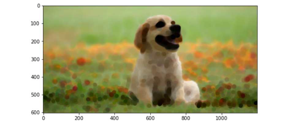
Gaussian Filter

The gaussian filter depends on the standard deviation of the image (distribution) and assumes the mean is zero (we can define a mean different from zero as well). Gaussian filters do not take care of the edges.

Value of certain statistical parameters defines the preservation. It is used for introductory image blurring. It generally works by defining a kernel. Suppose we define a 3 x 3 kernel. We apply this kernel to each and every pixel present in the image, and average the result, which results in a blurred image.

Cv2.GaussianBlur() is the function use to apply a gaussian filter. It has three parameters.

1 – The image, which needs to be blurred

2 – The size of the kernel (3 x 3 in this case)

3 – The standard deviation

Bilateral Filter

If we want to smooth an image and keep the edges intact, we use a bilateral filter. Its implementation is simple: we replace the pixel value with the average of its neighbors. This is a nonlinear smoothing approach that takes the weighted average of neighboring pixels. “Neighbors” are defined in following ways:

• Two pixel values are close to each other
• Two pixel values are similar to each other

Cv2.bilateralFilter has four parameters:

1. The image we want to smooth
2. The diameter of the pixel neighborhood (defining the neighborhood diameter to search for neighbors)
3. The sigma value for color (to find the pixels that are similar)
4. The sigma value for space 9to find the pixels that are closer)

Let’s take a look at the code:

Changing the Shape of Image

in this section we examine erosion and dilation, which are the two operations used to change the shape of images. Dilation results in the addition of pixels to the boundary of an object; erosion leads to the removal of pixels from the boundary.

Two erode or dilate an image, we first define the neighborhood kernel, which can be done in three ways:

1 – MORPH_RECT: to make a rectangular kernel.

2 – MORPH_CROSS: to make a cross-shaped kernel.

3 – MORPH_ELLIPS: to make an elliptical kernel.

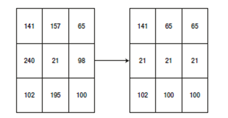
The kernel finds the neighbors of a pixel, which helps us in eroding or dilating an image. For dilation, the maximum value generates a new pixel value. For erosion, the minimum value.

in a kernel generates a new pixel value. In Figure 4-1, we apply a 3 × 1 matrix to find the minimum for each row. For the first element, the kernel starts from one cell before. Because the value is not present in the new cell to the left, we take it as blank. This concept is called padding. So, the first minimum is checked between none, 141 and 157. Thus, 141 is the minimum, and you see 141 as the first value in the right matrix. Then, the kernel shifts toward right. Now the cells to consider are 141, 157, and 65. This time, 65 is the minimum, so second value in the new matrix is 65. The third time, the kernel compares 157, 65, and none, because there is no third cell. Therefore, the minimum is 65 and that becomes the last value. This operation is performed for each and every cell, and you get the new matrix shown below:

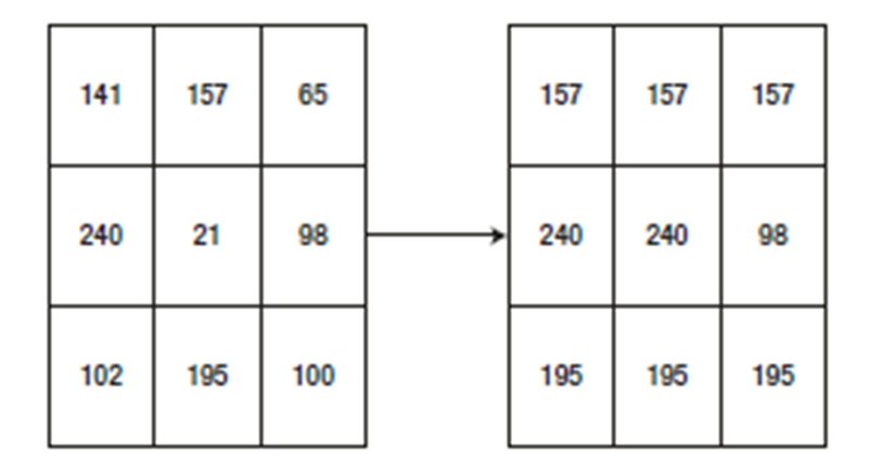
Dilation

The erosion operation is done similar to dilation, except instead of finding the minimum, we find the maximum.

Erosion

The kernel size is, an in dilation, a 3 x 1 rectangle.

Cv2.getStructuringElement() is the function used to define the kernel and pass it down to the erode or dilation function. Let’s see its parameters:

• Erosion/dilation type
• Kernel size
• Point at which the kernel should start

After applying cv2.getStructuringElement() and getting the final kernel, we use cv2.erode() and cv2.dilate() to perform the specific operation. Let’s look at the code and its output:

# Dilation code

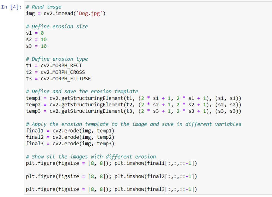
# Erosion code:

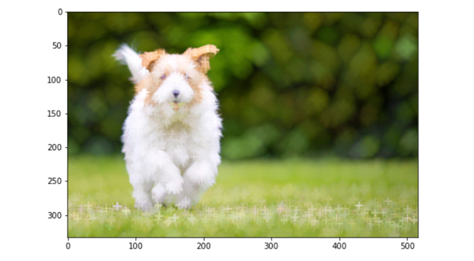
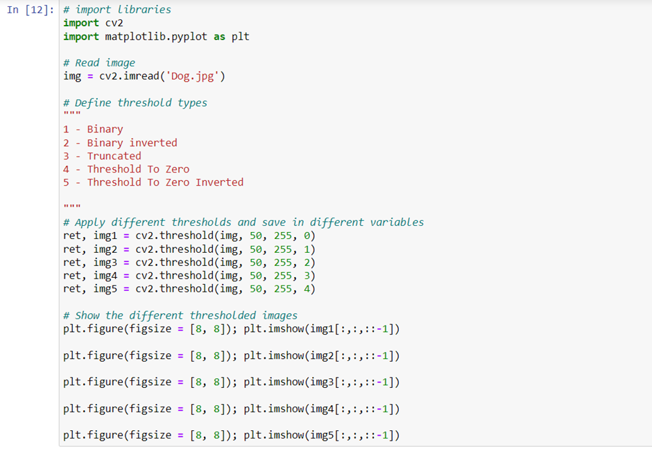
Effecting Image Thresholding

The main reason you would do image thresholding is to segment images. We try to get an object out of the image by removing the background and by focusing on the object. To do this, we first convert the image to grayscale and into a binary format—meaning, the image contains black or white only.

We provide a reference pixel value, and all the values above or below it are converted to black or white. There are five thresholding types:

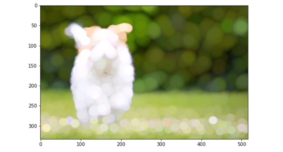
1. Binary: If the pixel value is greater than the reference pixel value (the threshold value), then convert to white (255); otherwise, convert to black (0).
   
2. Binary inverted: If the pixel value is greater than the reference pixel value (the threshold value), then convert to black (0); otherwise, convert to white (255). Just the opposite of the binary type.
   
3. Truncated: If the pixel value is greater than the reference pixel value (the threshold value), then convert to the threshold value; otherwise, don’t change the value.
   
4. Threshold to zero: If the pixel value is greater than the reference pixel value (the threshold value), then don’t change the value; otherwise convert to black (0).
   
5. Threshold to zero inverted: If the pixel value is greater than the reference pixel value (the threshold value), then convert to black (0); otherwise, don’t change. We use the cv2.threshold() function to do image thresholding, which uses the following parameters:

• The image to convert
• The threshold value
• The maximum pixel value
• The type of thresholding (as listed earlier)

Let’s look at the code and its output.

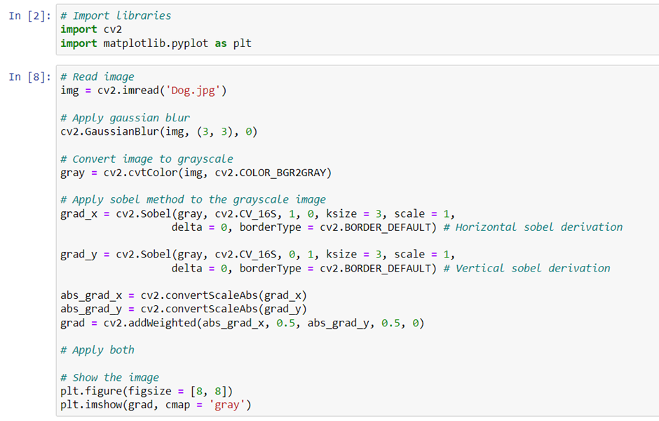
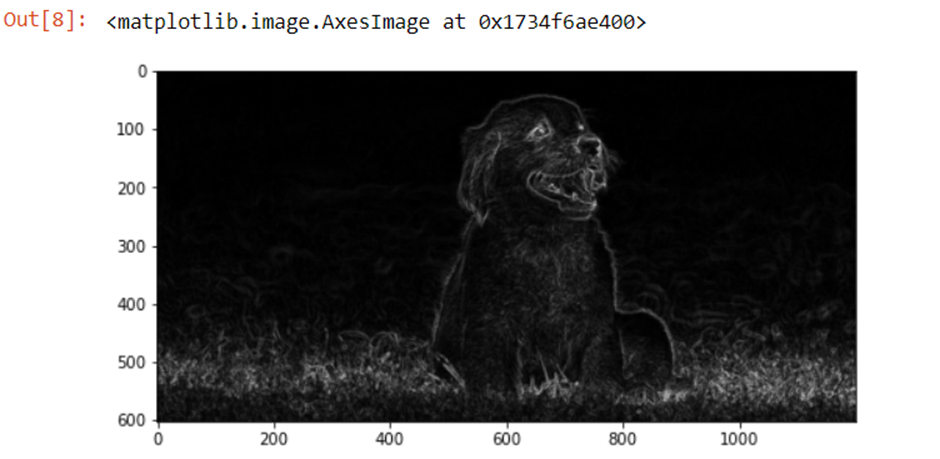
Calculating Gradients

In this section we look at edge detection using Sobel derivatives. Edges can be found in two directions either the vertical direction and the horizontal direction. With this algorithm, we emphasize only those regions that have very high spatial frequency, which may correspond to edges. Spatial frequency is the level of detail present in an area of importance.

In the below code, we will read the image, and apply gaussian blur so that the noise is removed, then will convert the image to grayscale. We use the cv2.cvtColor() function to convert the image to grayscale. We can also use some other library like skimage functions to do the same. Last, we give the grayscale output to the cv2.Sobel() function.

Let’s look at Sobel Function’s parameters:

• Input image
  
• Depth of the output image. The greater the depth of the image, the lesser the chances you miss any border. You can experiment with all of the below listed parameters, to see whether they capture the borders effectively, per your requirements. Depth can be of following types:
  
• –1 (the same depth as the original image)
  
• cv2.CV_16S
  
• cv2.CV_32F
  
• cv2.CV_64F
  
• Order of derivative x (defines the derivative order for finding horizontal edges)
  
• Order of derivative y (defines the derivative order for finding vertical edges)
  
• Size of the kernel
  
• Scale factor to be applied to the derivatives
  
• Delta value to be added as a scalar in the formula
  
• Border type for extrapolation of pixels

The cv2.convertScaleAbs() function is used to convert the values into an absolute number, with an unsigned 8-bit type. Then we blend the x and y gradients that we found to find the overall edges in the image. Let’s look at the code and its output.

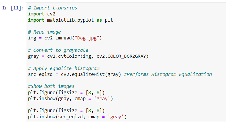
Histogram equalizer

Histogram equalization is used to adjust the contrast of an image. We first plot the histogram of pixel intensity distribution and then modify it. There is a cumulative probability function associated with every image. Histogram equalization gives linear trend to that function. We should use a grayscale image to perform histogram equalization. The cv2.equalizeHist() function is used for histogram equalization.

Let’s look at an example.

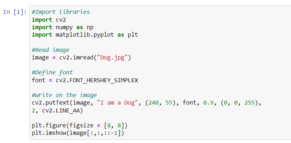
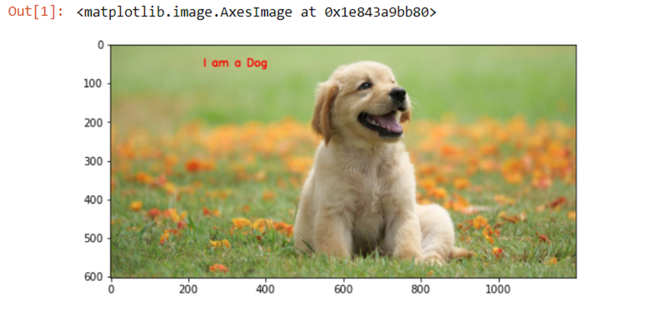
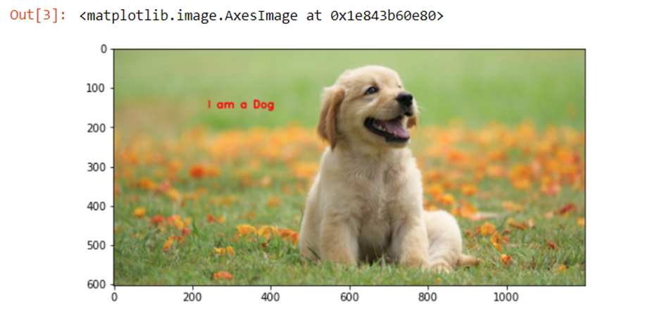
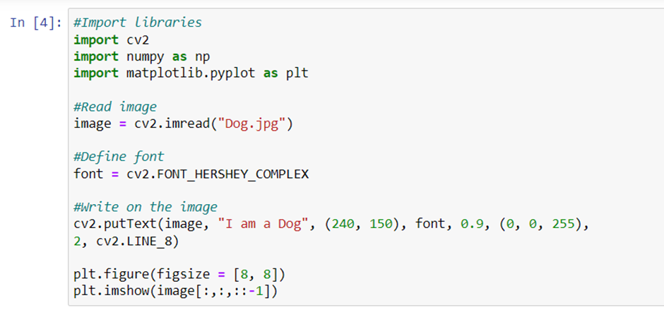
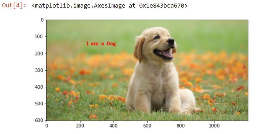
Adding text to image

cv2.putText() is a function present in the cv2 module that allows us to add text to images. The function takes following arguments:

• Image, where you want to write the text
• The text you want to write
• Position of the text on the image
• Font type
• Font scale
• Color of the text
• Thickness of text
• Type of line used

As you can see in the code that follows, the font used is FONT_HERSHEY_SIMPLEX. cv2 also supports following fonts:

• FONT_HERSHEY_SIMPLEX
• FONT_HERSHEY_PLAIN
• FONT_HERSHEY_DUPLEX
• FONT_HERSHEY_COMPLEX
• FONT_HERSHEY_TRIPLEX
• FONT_HERSHEY_COMPLEX_SMALL
• FONT_HERSHEY_SCRIPT_SIMPLEX
• FONT_HERSHEY_SCRIPT_COMPLEX
• FONT_ITALIC

The type of line that used in the code is cv2.LINE_AA. Other types of lines that are supported are

• FILLED: a completely filled line
• LINE_4: four connected lines
• LINE_8: eight connected lines
• LINE_AA: an anti-aliasing line

You can experiment using all the different arguments and check the results. Let’s look at the code and its output.

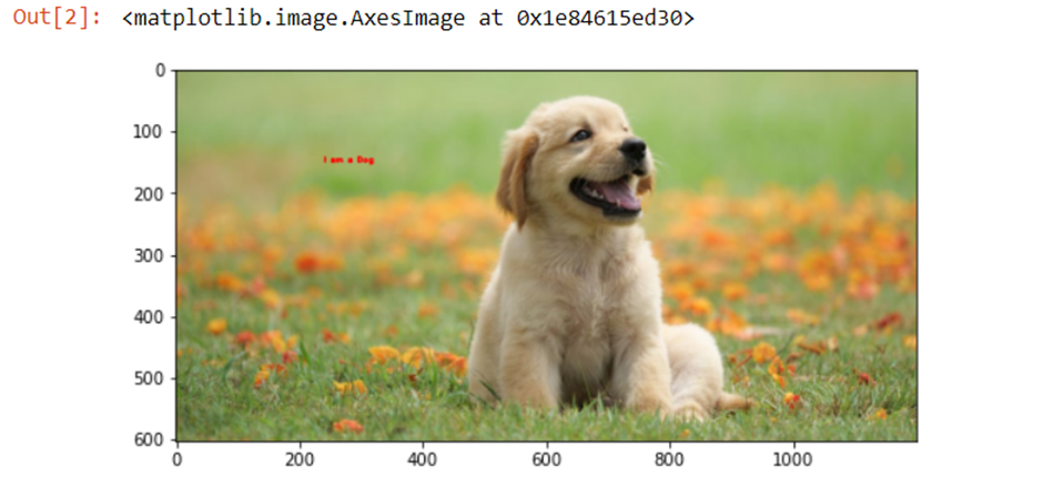
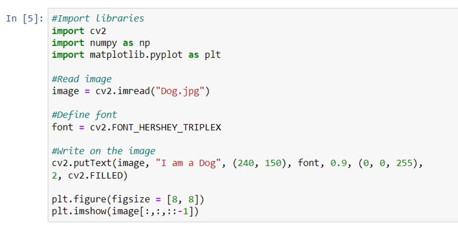
As you can see, we have used 5 different FONT method. You can try other methods also and check how the results are different from one other.

Popular Posts