Implementing Linear Regression from Scratch with Python

Linear regression is a fundamental machine learning algorithm that allows us to predict numerical values based on input data. In this article, we will see how to implement linear regression from scratch using Python. We will break down the code into simple steps, explaining each one along the way. So, let’s understand how linear regression works!

Linear Regression from Scratch using Python

Step 1: Importing the necessary libraries

To begin, we need to import the required libraries. In our code, we will use the NumPy library for numerical computations and data manipulation.

import numpy as np

Step 2: Creating the LinearRegression class

Next, we define a class called LinearRegression. Inside the class, we initialize various parameters such as learning rate (lr) and number of iterations (n_iters). Additionally, we define placeholders for weights and bias.

class LinearRegression:
    def __init__(self, lr=0.001, n_iters=1000):
        self.lr = lr
        self.n_iters = n_iters
        self.weights = None
        self.bias = None

Step 3: Training the model

In the fit() method of our LinearRegression class, we perform the training process. We first determine the number of samples and features in the input data (X). Then, we initialize the weights and bias to zeros.

def fit(self, X, y):
    n_samples, n_features = X.shape
    self.weights = np.zeros(n_features)
    self.bias = 0

Next, we iterate for the specified number of iterations. During each iteration, we make predictions by taking the dot product of the input data (X) and the weights, and add the bias term. Then, we calculate the gradients (dw and db) for the weights and bias, respectively, using the formulas derived from the gradient descent algorithm.

    for _ in range(self.n_iters):
        y_pred = np.dot(X, self.weights) + self.bias

        dw = (1/n_samples) * np.dot(X.T, (y_pred-y))
        db = (1/n_samples) * np.sum(y_pred-y)

Finally, we update the weights and bias by subtracting the learning rate multiplied by the gradients. This step helps the model gradually converge towards the optimal values.

        self.weights = self.weights - self.lr * dw
        self.bias = self.bias - self.lr * db

Step 4: Making predictions

To predict the output values, we implement the predict() method in our LinearRegression class. It takes the input data (X), performs the dot product with the weights, adds the bias, and returns the predicted values.

def predict(self, X):
    y_pred = np.dot(X, self.weights) + self.bias
    return y_pred

Now that we have gone through the steps for implementing linear regression, let’s move on to utilizing our code and visualizing the results.

Now, let’s create one more python file called “train.py” where we will import our “LinearRegression.py” file and train our model.

Step 1: Importing libraries

We start by importing additional libraries such as train_test_split from sklearn.model_selection, datasets from sklearn, and matplotlib.pyplot as plt. These libraries will help us with data splitting, generating a regression dataset, and visualizing the results.

import numpy as np
from sklearn.model_selection import train_test_split
from sklearn import datasets
import matplotlib.pyplot as plt
from LinearRegression import LinearRegression

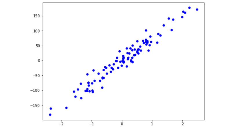
Step 2: Generating and visualizing the dataset

Using the datasets.make_regression() function, we generate a synthetic regression dataset with 100 samples and 1 feature. We then split the data into training and testing sets using train_test_split()

X, y = datasets.make_regression(n_samples=100, n_features=1, noise=20, random_state=4)
X_train, X_test, y_train, y_test = train_test_split(X, y, test_size=0.2, random_state=1234)

To visualize the dataset, we plot the scattered points using plt.scatter().

fig = plt.figure(figsize=(8,6))
plt.scatter(X[:, 0], y, color="b", marker="o", s=30)
plt.show()

Step 3: Training and evaluating the model

Now, we create an instance of our LinearRegression class and fit it to the training data using fit(). We then make predictions on the test data using predict().

reg = LinearRegression(lr=0.01)
reg.fit(X_train, y_train)
predictions = reg.predict(X_test)

Step 4: Evaluating the model’s performance

To evaluate the performance of our model, we define a mean squared error (MSE) function. It calculates the average squared difference between the predicted and actual values.

def mse(y_test, predictions):
    return np.mean((y_test - predictions) ** 2)

mse = mse(y_test, predictions)
print(mse)

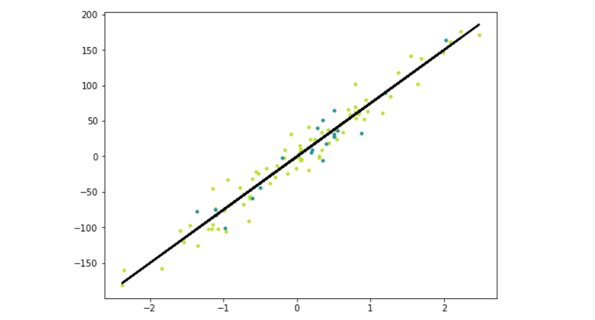
Step 5: Visualizing the regression line

To visualize the regression line, we generate predictions for the entire dataset and plot it alongside the training and testing data.

y_pred_line = reg.predict(X)
cmap = plt.get_cmap('viridis')
fig = plt.figure(figsize=(8,6))
m1 = plt.scatter(X_train, y_train, color=cmap(0.9), s=10)
m2 = plt.scatter(X_test, y_test, color=cmap(0.5), s=10)
plt.plot(X, y_pred_line, color='black', linewidth=2, label='Prediction')
plt.show()

Complete code:

import numpy as np


class LinearRegression:

    def __init__(self, lr = 0.001, n_iters=1000):
        self.lr = lr
        self.n_iters = n_iters
        self.weights = None
        self.bias = None

    def fit(self, X, y):
        n_samples, n_features = X.shape
        self.weights = np.zeros(n_features)
        self.bias = 0

        for _ in range(self.n_iters):
            y_pred = np.dot(X, self.weights) + self.bias

            dw = (1/n_samples) * np.dot(X.T, (y_pred-y))
            db = (1/n_samples) * np.sum(y_pred-y)

            self.weights = self.weights - self.lr * dw
            self.bias = self.bias - self.lr * db

    def predict(self, X):
        y_pred = np.dot(X, self.weights) + self.bias
        return y_pred

import numpy as np
from sklearn.model_selection import train_test_split
from sklearn import datasets
import matplotlib.pyplot as plt
from LinearRegression import LinearRegression

X, y = datasets.make_regression(n_samples=100, n_features=1, noise=20, random_state=4)
X_train, X_test, y_train, y_test = train_test_split(X, y, test_size=0.2, random_state=1234)

fig = plt.figure(figsize=(8,6))
plt.scatter(X[:, 0], y, color = "b", marker = "o", s = 30)
plt.show()

reg = LinearRegression(lr=0.01)
reg.fit(X_train,y_train)
predictions = reg.predict(X_test)

def mse(y_test, predictions):
    return np.mean((y_test-predictions)**2)

mse = mse(y_test, predictions)
print(mse)

y_pred_line = reg.predict(X)
cmap = plt.get_cmap('viridis')
fig = plt.figure(figsize=(8,6))
m1 = plt.scatter(X_train, y_train, color=cmap(0.9), s=10)
m2 = plt.scatter(X_test, y_test, color=cmap(0.5), s=10)
plt.plot(X, y_pred_line, color='black', linewidth=2, label='Prediction')
plt.show()

And that’s it! We have successfully implemented linear regression from scratch using Python. We saw each step along the way, allowing you to understand the code and its functionality.

Linear regression is a powerful and widely used algorithm for predicting continuous values. By building it from scratch, you gain a deeper understanding of its inner workings of it.

If you found this article helpful and insightful, I would greatly appreciate your support. You can show your appreciation by clicking on the button below. Thank you for taking the time to read this article.

Nomidl