Brain tumor detection plays an important role in diagnosing and treating brain-related diseases. With advancements in machine learning and image processing techniques, it is now possible for us to automate the process of tumor detection using computer algorithms. In this article, we will look at the code implementation that uses machine learning models to detect brain tumors from MRI images. We will help you to understand the code step-by-step, explaining the underlying concepts and providing insights into the evaluation and visualization of the results.

Step 1: Setting up the Directory and Class Labels
The first step in our code is to import necessary libraries and define the directory where the training images are stored and specify the class labels. In our case, we have two classes: ‘no_tumor’ and ‘pituitary_tumor’. This step ensures that the code knows where to find the images and how to assign the corresponding labels for training.
import numpy as np
import pandas as pd
import matplotlib.pyplot as plt
from sklearn.model_selection import train_test_split
from sklearn.metrics import accuracy_score
import os
import cv2
from sklearn.linear_model import LogisticRegression
from sklearn.svm import SVC
import warnings

# Set up the directory and class labels
path = os.listdir('brain_tumor/Training/')
classes = {'no_tumor': 0, 'pituitary_tumor': 1}
Step 2: Loading and Preprocessing the Images
Next, we load the images from the training directory and preprocess them. The code iterates through each class and reads the images using the OpenCV library. The images are resized to a consistent dimension of 200×200 pixels to ensure uniformity. The pixel intensities are then stored in the ‘X’ array, and the corresponding class labels are stored in the ‘Y’ array. This process prepares the data for training the machine learning models.
# Load and preprocess the images
X = []
Y = []
for cls in classes:
    pth = 'brain_tumor/Training/' + cls
    for j in os.listdir(pth):
        img = cv2.imread(pth + '/' + j, 0)
        img = cv2.resize(img, (200, 200))
        X.append(img)
        Y.append(classes[cls])

X = np.array(X)
Y = np.array(Y)
Step 3: Reshaping and Splitting the Data
To feed the image data into the machine learning models, we reshape the ‘X’ array to have a 2D shape, where each row represents an image and each column represents a flattened pixel. Additionally, we split the data into training and testing sets using the ‘train_test_split’ function from the ‘sklearn.model_selection’ module. This separation ensures that we have a separate set of images to evaluate the performance of our trained models.
# Reshape the data and split into training and testing sets
X_updated = X.reshape(len(X), -1)
xtrain, xtest, ytrain, ytest = train_test_split(X_updated, Y, random_state=10, test_size=.20)
Step 4: Normalizing the Pixel Values
To ensure that the pixel values of the images are within a consistent range, we normalize them. This step involves dividing each pixel value by 255, which scales the values between 0 and 1. Normalizing the data helps in improving the convergence of machine learning algorithms and ensures fair comparison across different features.
# Normalize the pixel values
xtrain = xtrain / 255
xtest = xtest / 255
Step 5: Training the Models
In this step, we train two different machine learning models: Logistic Regression and Support Vector Machines (SVM). We initialize the models and fit them to the training data. Logistic Regression is a classification algorithm that models the probability of a sample belonging to a particular class. SVM, on the other hand, finds an optimal hyperplane to separate the classes in a high-dimensional space. The ‘warnings’ module is used to suppress any potential warnings during the training process.
# Train the models
warnings.filterwarnings('ignore')
lg = LogisticRegression(C=0.1)
lg.fit(xtrain, ytrain)

sv = SVC()
sv.fit(xtrain, ytrain)
Step 6: Evaluating the Models
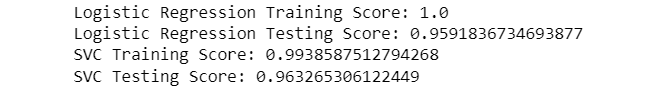
Once the models are trained, we evaluate their performance using the training and testing data. We calculate the training and testing scores for both the Logistic Regression and SVM models. These scores indicate how well the models have learned to classify the brain tumor images. A higher score indicates better accuracy.
# Evaluate the models
lg_train_score = lg.score(xtrain, ytrain)
lg_test_score = lg.score(xtest, ytest)

sv_train_score = sv.score(xtrain, ytrain)
sv_test_score = sv.score(xtest, ytest)

# Print the scores
print("Logistic Regression Training Score:", lg_train_score)
print("Logistic Regression Testing Score:", lg_test_score)
print("SVC Training Score:", sv_train_score)
print("SVC Testing Score:", sv_test_score)
Step 7: Predicting on Test Data
After evaluating the models, we use the trained SVM model to predict the class labels for the test data. The predictions are stored in the ‘pred’ variable, and we identify the misclassified samples by comparing the predicted labels with the true labels.
# Predict on test data
pred = sv.predict(xtest)
misclassified = np.where(ytest != pred)

# Print misclassified samples
print("Total Misclassified Samples: ", len(misclassified[0]))
print("Predicted Label:", pred[36])
print("True Label:", ytest[36])

# Define label decoding
label_decoder = {0: 'No Tumor', 1: 'Positive Tumor'}

Step 8: Visualization of Results
To visually inspect the results, we plot a selection of test images along with their predicted labels. We iterate through the test images in both the ‘no_tumor’ and ‘pituitary_tumor’ classes, display the images using the ‘imshow’ function from the ‘matplotlib.pyplot’ library, and assign the corresponding predicted labels using the ‘label_decoder’ dictionary. This allows us to see the model’s predictions and compare them with the actual images.
# Plot test images with predictions
plt.figure(figsize=(12, 8))
p = os.listdir('brain_tumor/Testing/')
c = 1
for i in os.listdir('brain_tumor/Testing/no_tumor/')[:9]:
    plt.subplot(3, 3, c)
    img = cv2.imread('brain_tumor/Testing/no_tumor/' + i, 0)
    img1 = cv2.resize(img, (200, 200))
    img1 = img1.reshape(1, -1) / 255
    p = sv.predict(img1)
    plt.title(label_decoder[p[0]])
    plt.imshow(img, cmap='gray')
    plt.axis('off')
    c += 1

plt.figure(figsize=(12, 8))
p = os.listdir('brain_tumor/Testing/')
c = 1
for i in os.listdir('brain_tumor/Testing/pituitary_tumor/')[:16]:
    plt.subplot(4, 4, c)
    img = cv2.imread('brain_tumor/Testing/pituitary_tumor/' + i, 0)
    img1 = cv2.resize(img, (200, 200))
    img1 = img1.reshape(1, -1) / 255
    p = sv.predict(img1)
    plt.title(label_decoder[p[0]])
    plt.imshow(img, cmap='gray')
    plt.axis('off')
    c += 1

Conclusion
In this article, we explored a code implementation for detecting brain tumors using machine learning techniques. We walked through each step, starting from setting up the directory and class labels, to loading and preprocessing the images, reshaping and splitting the data, normalizing the pixel values, training the models, evaluating their performance, predicting on test data, and finally visualizing the results.
I hope you liked this article, let me know if you have any question.