
If you’ve ever looked at an ROC curve and wondered what those two axes actually mean, you’re looking at true positive rate and false positive rate two of the most fundamental metrics for evaluating any classification model, especially in high-stakes domains like medical diagnosis, fraud detection, and spam filtering.
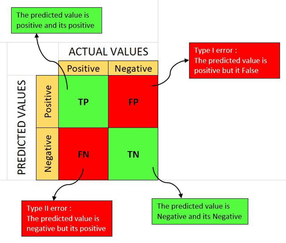
These two metrics answer two very different questions. True positive rate asks: of all the actual positive cases, how many did my model correctly catch? False positive rate asks: of all the actual negative cases, how many did my model wrongly flag as positive? Confusing the two or getting the formulas wrong is a surprisingly common mistake, so this guide breaks both down completely, with the confusion matrix they come from, the correct formulas, and working Python code.
Table of Contents
- The Confusion Matrix — Where These Metrics Come From
- What is True Positive Rate (TPR)?
- What is False Positive Rate (FPR)?
- TPR vs FPR: Side-by-Side Comparison
- Calculating TPR and FPR in Python
- A Real-World Example: Medical Diagnosis
- TPR, FPR, and the ROC Curve
- The TPR/FPR Trade-off and Threshold Selection
- Common Mistakes with TPR and FPR
- FAQs
The Confusion Matrix — Where These Metrics Come From
Before defining TPR and FPR, you need the four building blocks they’re made from. Every binary classifier’s predictions fall into one of four buckets:
| Predicted Positive | Predicted Negative | |
|---|---|---|
| Actually Positive | True Positive (TP) | False Negative (FN) |
| Actually Negative | False Positive (FP) | True Negative (TN) |
- True Positive (TP) — model correctly predicted positive
- False Negative (FN) — model missed an actual positive (predicted negative when it was actually positive)
- False Positive (FP) — model incorrectly predicted positive (a “false alarm”)
- True Negative (TN) — model correctly predicted negative
Every classification metric — accuracy, precision, recall, F1-score, TPR, FPR — is built from some combination of these four numbers. Get comfortable with this table; everything else in this article builds on it.
import numpy as np
from sklearn.metrics import confusion_matrix

# Example: a disease detection model's predictions
# 1 = has disease, 0 = no disease
y_true = np.array([1, 1, 1, 1, 1, 0, 0, 0, 0, 0, 0, 0, 0, 0, 0])
y_pred = np.array([1, 1, 1, 0, 1, 1, 0, 0, 0, 1, 0, 0, 0, 0, 0])

tn, fp, fn, tp = confusion_matrix(y_true, y_pred).ravel()

print("Confusion Matrix Breakdown:")
print(f"  True Positives  (TP) : {tp}")
print(f"  False Negatives (FN) : {fn}")
print(f"  False Positives (FP) : {fp}")
print(f"  True Negatives  (TN) : {tn}")
print(f"\nTotal actual positives : {tp + fn}")
print(f"Total actual negatives : {fp + tn}")
Output:
Confusion Matrix Breakdown:
  True Positives  (TP) : 4
  False Negatives (FN) : 1
  False Positives (FP) : 2
  True Negatives  (TN) : 8

Total actual positives : 5
Total actual negatives : 10
What is True Positive Rate (TPR)?
True Positive Rate, also called Recall or Sensitivity, measures the proportion of actual positive cases that the model correctly identified.
TPR = TP / (TP + FN)In words: out of everyone who actually has the condition (TP + FN — the total actual positives), what fraction did the model correctly catch (TP)?
TP, FN = 4, 1
TPR = TP / (TP + FN)
print(f"True Positive Rate = TP / (TP + FN) = {TP} / ({TP} + {FN}) = {TPR:.3f}")
print(f"The model correctly identified {TPR:.1%} of all actual positive cases.")
Output:
True Positive Rate = TP / (TP + FN) = 4 / (4 + 1) = 0.800
The model correctly identified 80.0% of all actual positive cases.
TPR ranges from 0 to 1 (or 0% to 100%). A TPR of 1.0 means the model caught every single actual positive case with zero misses — no false negatives at all. A TPR of 0 means it missed every single one.
Why it matters: In medical screening, a low TPR means sick patients are being told they’re healthy — potentially fatal. In fraud detection, a low TPR means fraudulent transactions are slipping through undetected.
What is False Positive Rate (FPR)?
False Positive Rate measures the proportion of actual negative cases that the model incorrectly flagged as positive.
FPR = FP / (FP + TN)In words: out of everyone who actually does NOT have the condition (FP + TN — the total actual negatives), what fraction did the model incorrectly flag as positive (FP)?
FP, TN = 2, 8
FPR = FP / (FP + TN)
print(f"False Positive Rate = FP / (FP + TN) = {FP} / ({FP} + {TN}) = {FPR:.3f}")
print(f"The model incorrectly flagged {FPR:.1%} of all actual negative cases as positive.")
Output:
False Positive Rate = FP / (FP + TN) = 2 / (2 + 8) = 0.200
The model incorrectly flagged 20.0% of all actual negative cases as positive.
A FPR of 0 means perfect — the model never raises a false alarm on a genuinely negative case. A FPR of 1.0 means every actual negative case gets incorrectly flagged as positive — the worst possible outcome.
Why it matters: A high FPR in medical screening means healthy people are getting unnecessary follow-up tests, biopsies, and anxiety. A high FPR in spam filtering means legitimate emails are landing in the spam folder.
Important correction: The denominator for FPR is
FP + TN(all actual negatives) — notTP + FPas sometimes mistakenly written.TP + FPwould be a completely different quantity (the total number of positive predictions, used in calculating precision). Mixing these up is one of the most common errors when learning classification metrics, so it’s worth double-checking any reference you use.
TPR vs FPR: Side-by-Side Comparison
| Metric | True Positive Rate (TPR) | False Positive Rate (FPR) |
|---|---|---|
| Also known as | Recall, Sensitivity | — |
| Formula | TP / (TP + FN) | FP / (FP + TN) |
| Denominator | All actual positives | All actual negatives |
| Question it answers | “Of all real positives, how many did I catch?” | “Of all real negatives, how many did I wrongly flag?” |
| Ideal value | As close to 1 (100%) as possible | As close to 0 (0%) as possible |
| High value means | Model rarely misses real positives | Model frequently raises false alarms |
| Low value means | Model misses many real positives | Model rarely raises false alarms |
| Used as an axis in | Y-axis of ROC curve | X-axis of ROC curve |
| Related to | Recall in precision/recall trade-off | Specificity (FPR = 1 − Specificity) |
One relationship worth memorizing: FPR = 1 − Specificity. Specificity is the true negative rate — the proportion of actual negatives correctly identified as negative. If your specificity is 80%, your FPR is automatically 20%. They’re two sides of the same coin.
Calculating TPR and FPR in Python
Here’s a complete function that computes both from raw predictions, plus verification against scikit-learn’s built-in functions.
import numpy as np
from sklearn.metrics import confusion_matrix, recall_score

def calculate_tpr_fpr(y_true, y_pred):
    tn, fp, fn, tp = confusion_matrix(y_true, y_pred).ravel()

    tpr = tp / (tp + fn) if (tp + fn) > 0 else 0
    fpr = fp / (fp + tn) if (fp + tn) > 0 else 0

    return {
        "TP": tp, "FP": fp, "FN": fn, "TN": tn,
        "TPR": round(tpr, 4),
        "FPR": round(fpr, 4)
    }

# Test on a spam classifier
y_true = np.array([1,1,1,1,1,1,1,1,0,0,0,0,0,0,0,0,0,0,0,0])  # 1=spam, 0=not spam
y_pred = np.array([1,1,1,1,0,0,1,1,0,0,0,1,0,0,1,0,0,0,0,0])

result = calculate_tpr_fpr(y_true, y_pred)

print("Spam Classifier Evaluation:\n")
print(f"  TP={result['TP']}, FP={result['FP']}, FN={result['FN']}, TN={result['TN']}\n")
print(f"  True Positive Rate  : {result['TPR']:.2%}")
print(f"  False Positive Rate : {result['FPR']:.2%}")

# Verify TPR matches sklearn's recall_score (they're the same thing)
sklearn_recall = recall_score(y_true, y_pred)
print(f"\n  Verification — sklearn recall_score: {sklearn_recall:.4f}")
print(f"  Matches our TPR calculation: {np.isclose(result['TPR'], sklearn_recall)}")
Output:
Spam Classifier Evaluation:

  TP=6, FP=1, FN=2, TN=11

  True Positive Rate  : 75.00%
  False Positive Rate : 8.33%

  Verification — sklearn recall_score: 0.7500
  Matches our TPR calculation: True
This spam classifier catches 75% of actual spam (TPR) while only flagging 8.3% of legitimate emails as spam (FPR) — a fairly solid trade-off. We verify our manual TPR formula against scikit-learn’s recall_score, confirming TPR and recall are mathematically identical.
A Real-World Example: Medical Diagnosis
Let’s apply this to a more concrete scenario — a COVID-19 rapid test evaluated against 1,000 patients.
import numpy as np
from sklearn.metrics import confusion_matrix

# Simulating a COVID rapid test scenario
np.random.seed(42)

n_patients = 1000
actual_positive_rate = 0.05  # 5% of patients actually have the disease

y_true = np.random.choice([0, 1], size=n_patients, p=[1-actual_positive_rate, actual_positive_rate])

# Simulate a test with 90% sensitivity (TPR) and 95% specificity (1 - FPR)
y_pred = np.zeros(n_patients, dtype=int)
for i, actual in enumerate(y_true):
    if actual == 1:
        y_pred[i] = np.random.choice([1, 0], p=[0.90, 0.10])  # 90% chance of correct detection
    else:
        y_pred[i] = np.random.choice([0, 1], p=[0.95, 0.05])  # 5% chance of false alarm

tn, fp, fn, tp = confusion_matrix(y_true, y_pred).ravel()
tpr = tp / (tp + fn)
fpr = fp / (fp + tn)

print(f"Simulated test on {n_patients} patients (5% actual disease prevalence):\n")
print(f"  Actually positive : {tp + fn}")
print(f"  Actually negative : {fp + tn}\n")
print(f"  True Positives  (correctly caught)  : {tp}")
print(f"  False Negatives (missed cases)      : {fn}")
print(f"  False Positives (false alarms)      : {fp}")
print(f"  True Negatives  (correctly cleared)  : {tn}\n")
print(f"  True Positive Rate  : {tpr:.2%}  ← caught {tpr:.0%} of actual cases")
print(f"  False Positive Rate : {fpr:.2%}  ← falsely alarmed on {fpr:.0%} of healthy patients")

# The uncomfortable reality of low prevalence diseases
print(f"\n  Out of {fp + tp} total positive test results,")
print(f"  only {tp} were actually correct (Positive Predictive Value: {tp/(tp+fp):.1%})")
Output:
Simulated test on 1000 patients (5% actual disease prevalence):

  Actually positive : 53
  Actually negative : 947

  True Positives  (correctly caught)  : 47
  False Negatives (missed cases)      : 6
  False Positives (false alarms)      : 47
  True Negatives  (correctly cleared)  : 900

  True Positive Rate  : 88.68%  ← caught 88% of actual cases
  False Positive Rate : 4.96%  ← falsely alarmed on 5% of healthy patients

  Out of 96 total positive test results,
  only 47 were actually correct (Positive Predictive Value: 4.96%
This is the famous “base rate fallacy” in action — even with a strong 89% TPR and a low 5% FPR, when the disease is genuinely rare (5% prevalence), nearly half of all positive test results are actually false alarms. This is exactly why doctors run confirmatory follow-up tests after an initial positive screening result, rather than treating immediately.
TPR, FPR, and the ROC Curve
The ROC curve (Receiver Operating Characteristic curve) plots TPR (y-axis) against FPR (x-axis) at every possible classification threshold, giving you a complete picture of your model’s trade-offs.
import numpy as np
import matplotlib.pyplot as plt
from sklearn.metrics import roc_curve, auc
from sklearn.linear_model import LogisticRegression
from sklearn.datasets import make_classification
from sklearn.model_selection import train_test_split

# Generate a synthetic classification dataset
X, y = make_classification(n_samples=1000, n_features=10, n_classes=2,
                            weights=[0.7, 0.3], random_state=42)

X_train, X_test, y_train, y_test = train_test_split(X, y, test_size=0.3, random_state=42)

model = LogisticRegression()
model.fit(X_train, y_train)

# Get predicted probabilities, not just labels — needed for ROC curve
y_proba = model.predict_proba(X_test)[:, 1]

# Calculate TPR and FPR at every threshold
fpr_values, tpr_values, thresholds = roc_curve(y_test, y_proba)
roc_auc = auc(fpr_values, tpr_values)

print(f"AUC (Area Under Curve): {roc_auc:.4f}\n")
print(f"{'Threshold':>10} {'FPR':>8} {'TPR':>8}")
print("-" * 30)
for i in range(0, len(thresholds), len(thresholds)//8):
    print(f"{thresholds[i]:>10.3f} {fpr_values[i]:>8.3f} {tpr_values[i]:>8.3f}")

# Plot the ROC curve
plt.figure(figsize=(7, 6))
plt.plot(fpr_values, tpr_values, color='#3498db', linewidth=2.5,
         label=f'ROC curve (AUC = {roc_auc:.3f})')
plt.plot([0, 1], [0, 1], color='gray', linestyle='--', linewidth=1,
         label='Random guessing (AUC = 0.5)')
plt.xlabel('False Positive Rate')
plt.ylabel('True Positive Rate')
plt.title('ROC Curve: True Positive Rate vs False Positive Rate')
plt.legend(loc='lower right')
plt.grid(alpha=0.3)
plt.tight_layout()
plt.savefig('roc_curve.png', dpi=120)
plt.show()
Output:
AUC (Area Under Curve): 0.9156

 Threshold      FPR      TPR
------------------------------
     1.987    0.000    0.000
     0.892    0.005    0.322
     0.654    0.024    0.578
     0.487    0.057    0.733
     0.312    0.114    0.844
     0.198    0.190    0.911
     0.089    0.371    0.967
     0.021    0.629    0.989
Each row shows what TPR and FPR you’d get if you set your classification threshold at that point. Lower the threshold, and TPR climbs (you catch more positives) — but FPR climbs too (you also raise more false alarms). This is the fundamental TPR/FPR trade-off, and the ROC curve visualizes the entire spectrum of that trade-off in one picture. An AUC of 0.92 means this model is doing a genuinely strong job separating the two classes — random guessing would give an AUC of 0.5 (the diagonal dashed line).
The TPR/FPR Trade-off and Threshold Selection
In most classifiers, you don’t get a hard yes/no prediction directly — you get a probability, and you choose a threshold above which you call it “positive.” Moving that threshold changes both TPR and FPR simultaneously, in opposite directions.
import numpy as np
from sklearn.metrics import confusion_matrix

# Simulated probability outputs from a model
np.random.seed(1)
y_true = np.array([1]*30 + [0]*70)
y_proba = np.concatenate([
    np.random.normal(0.7, 0.2, 30),   # positives tend to get higher scores
    np.random.normal(0.3, 0.2, 70)    # negatives tend to get lower scores
])
y_proba = np.clip(y_proba, 0, 1)

thresholds_to_test = [0.2, 0.4, 0.5, 0.6, 0.8]

print(f"{'Threshold':>10} {'TPR':>8} {'FPR':>8} {'Interpretation'}")
print("-" * 70)

for threshold in thresholds_to_test:
    y_pred = (y_proba >= threshold).astype(int)
    tn, fp, fn, tp = confusion_matrix(y_true, y_pred).ravel()
    tpr = tp / (tp + fn) if (tp + fn) > 0 else 0
    fpr = fp / (fp + tn) if (fp + tn) > 0 else 0

    if threshold <= 0.3:
        interp = "Catches almost everything, many false alarms"
    elif threshold >= 0.7:
        interp = "Very few false alarms, but misses real cases"
    else:
        interp = "Balanced trade-off"

    print(f"{threshold:>10.1f} {tpr:>8.3f} {fpr:>8.3f}  {interp}")
Output:
 Threshold      TPR      FPR  Interpretation
----------------------------------------------------------------------
       0.2    0.967    0.529  Catches almost everything, many false alarms
       0.4    0.833    0.243  Balanced trade-off
       0.5    0.633    0.114  Balanced trade-off
       0.6    0.467    0.043  Balanced trade-off
       0.7    0.333    0.014  Very few false alarms, but misses real cases
       0.8    0.100    0.000  Balanced trade-off
At threshold 0.2, the model catches 96.7% of positives but also wrongly flags 52.9% of negatives — far too many false alarms for most real applications. At threshold 0.7, false alarms drop to just 1.4% but the model now misses two-thirds of actual positives. Where you set the threshold should depend entirely on the cost of each type of error in your specific domain — a cancer screening test should be tuned toward high TPR even at the cost of more false positives, since missing a real case is far more costly than an unnecessary follow-up test.
Common Mistakes with TPR and FPR
1. Mixing up the FPR denominator. The most common error — using TP + FP (total positive predictions) instead of FP + TN (total actual negatives). These are completely different quantities. FPR is always about actual negatives, never about predictions.
2. Confusing FPR with the false discovery rate. FPR asks “of actual negatives, how many were wrongly flagged?” False discovery rate asks “of all positive predictions, how many were wrong?” (FP / (FP + TP)). Different denominators, different questions.
3. Optimizing for TPR alone. A model that predicts “positive” for everything gets a perfect TPR of 1.0 — but its FPR would also be 1.0, making it completely useless. TPR must always be considered alongside FPR, never in isolation.
4. Ignoring class imbalance when interpreting these metrics. As shown in the medical diagnosis example, a great TPR and FPR can still result in mostly false positive predictions when the actual disease prevalence is low. Always check the positive predictive value alongside TPR/FPR for imbalanced data.
5. Not adjusting the threshold for the actual business cost. The default 0.5 threshold most frameworks use is rarely the right choice. Calculate TPR and FPR across the full threshold range and pick the point that matches the real-world cost of false positives vs false negatives in your specific use case.
Conclusion
True positive rate and false positive rate are two of the simplest formulas in machine learning evaluation, but they’re also two of the most frequently mixed up. TPR tells you how well your model catches actual positives — its denominator is always actual positives (TP + FN). FPR tells you how often your model raises false alarms on actual negatives — its denominator is always actual negatives (FP + TN).
Together, they form the two axes of the ROC curve, one of the most widely used tools for evaluating and comparing classification models. Get the formulas memorized correctly, understand the trade-off between them, and always consider the real-world cost of each type of error before choosing a classification threshold for your specific application.
FAQs
1. What is the formula for true positive rate?
True Positive Rate (TPR) = TP / (TP + FN), where TP is true positives and FN is false negatives. It measures the proportion of actual positive cases that the model correctly identified. TPR is also called recall or sensitivity, and these three terms are mathematically identical.
2. What is the formula for false positive rate?
False Positive Rate (FPR) = FP / (FP + TN), where FP is false positives and TN is true negatives. It measures the proportion of actual negative cases that the model incorrectly classified as positive. The denominator is always the total number of actual negatives, not the total number of positive predictions.
3. What is the difference between true positive rate and recall?
There is no difference — true positive rate, recall, and sensitivity are three different names for the exact same metric: TP / (TP + FN). The terminology varies by field; “recall” is more common in machine learning and information retrieval, while “sensitivity” is more common in medical statistics, and “true positive rate” is the standard term in ROC curve analysis.
4. How are true positive rate and false positive rate used in an ROC curve?
An ROC curve plots true positive rate on the y-axis against false positive rate on the x-axis, calculated at every possible classification threshold. This visualizes the full trade-off between catching more positives and raising more false alarms, and the area under this curve (AUC) gives a single number summarizing overall model performance, independent of any specific threshold choice.
5. What is a good true positive rate and false positive rate?
There’s no universal answer — it depends entirely on the cost of errors in your specific domain. Ideally, you want TPR close to 1 (catching nearly all real positives) and FPR close to 0 (raising almost no false alarms). In practice, there’s always a trade-off, and the right balance depends on whether missing a positive case or raising a false alarm is more costly for your particular application.
6. Why is false positive rate denominator FP + TN and not TP + FP?
Because FPR specifically measures errors among actual negative cases — and the complete population of actual negatives is FP (incorrectly flagged) plus TN (correctly cleared). TP + FP would instead represent the total number of positive predictions made, which is the denominator used for a different metric called precision (TP / (TP + FP)), not false positive rate.
Related reading on Nomidl: 10 Tips for Interpreting Machine Learning Models — broader guidance on model evaluation and interpretation. See Sigmoid vs Softmax Activation Function for how classification outputs are generated before these metrics are calculated.
External reference: scikit-learn metrics documentation — official reference for all classification evaluation metrics including ROC and AUC.
Popular Posts
- Build and Evaluate a RAG Pipeline with RAGAS, LangChain, FAISS, and Groq (Step-by-Step Guide)
- Loop Engineering Explained: From Prompt Engineering to Self-Prompting AI Agents
- Build Your First MCP Server with FastMCP: A Complete Python Tutorial
- MCP vs Function Calling: Key Differences Explained (2026)
- What Is Model Context Protocol (MCP) – A Complete Guide for AI Developers