Convolutional Neural Networks
CNN’s popularly known as ConvNets majority consists of several layers and are specifically used for image processing and detection of objects. It was developed in 1998 by Yann LeCun. CNNs have wide usage in identifying the image of the satellites, medical image processing, series forecasting, and anomaly detection.
CNNs process the data by passing it through multiple layers and extracting features to exhibit convolutional operations. The Convolutional Layer consists of Rectifies Linear Unit (ReLU) that outlasts to rectify the feature map. The Pooling layer is used to rectify these feature maps into the next feed. Pooling is generally a sampling algorithm that is down-sampled and it reduces the dimensions of the feature map. Later, the result generated consists of 2-D arrays consisting of single, long, continuous, and linear vector flattened in the map. The next layer i.e., called Fully Connected Layer which forms the flattened matrix or 2-D array fetched from the pooling layer as input and identifies the image by classifying it.

Long Short-Term Memory Networks
LSTM’S can be defined as Recurrent Neural Networks (RNN) that are programmed to learn and adapt for dependencies for the long term. It can memorize and recall past data for a greater period and by default, it is its sole behavior. LSTMs are designed to retain over time and henceforth they are majorly used in time series predictions because they can restrain memory or previous inputs. This analogy comes from their chain-like structure consisting of four interacting layers that communicate with each other differently. Besides applications of time series prediction, they can be used to construct speech recognizers, development in pharmaceuticals, and composition of music loops as well.
LSTM work in a sequence of events. First, they don’t tend to remember irrelevant details attained in the previous state. Next, they update certain cell-state values selectively and finally generate certain parts of the cell-state as output. Below is the diagram of their operation.

Recurrent Neural Networks
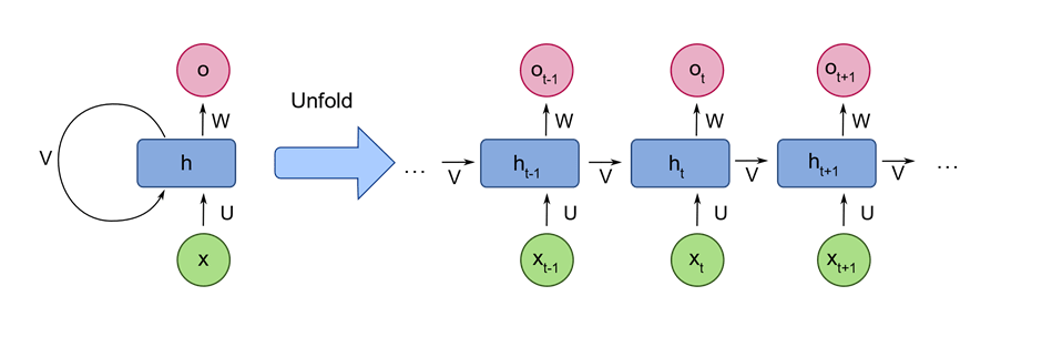
Recurrent Neural Networks or RNNs consist of some directed connections that form a cycle that allow the input provided from LSTMs to be used as input in the current phase of RNNs. These inputs are deeply embedded as inputs and enforce the memorization ability of LSTMs lets these inputs get absorbed for a period in the internal memory. RNNs are therefore dependent on the inputs that are preserved by LSTMs and work under the synchronization phenomenon of LSTMs. RNNs are mostly used in captioning the image, time series analysis, recognizing handwritten data, and translating data to machines.
RNNs follow the work approach by putting output feeds (t-1) time if the time is defined as t. next, the output determined by t is feed at input time t+1. Similarly, these processes are repeated for all the input consisting of any length. Theres is also a fact about RNNs is that they store historical information and there’s no increase in the input size even if the model size is increased. RNNs look something like when unfolded.
Generative Adversarial Networks
GANs are defined as deep learning algorithm that are used to generate new instances of data that match the training data. Over some time, GANs have gained immense usage since they are frequently being used to clarify astronomical images and simulate lensing the gravitational dark matter. It is also used in video games to increase graphics for 2D textures by recreating them in higher resolution like 4K. they are also used in creating realistic cartoons character and also rendering human faces and 3D object rendering.
GANs work in simulation by generating and understanding the fake data and the real data. During the training to understand these data, the generator produces different kinds of fake data where the discriminator quickly learns to adapt and respond to it as false data. GANs then used these recognized results of updating. Consider the below image to visualize the functioning.

Radial Basis Function Networks
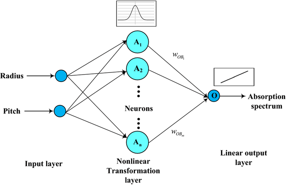
RBFNs are specific types of neural networks that follow a feed-forward approach and make use of radical functions as activation functions. They are mostly used for time-series prediction, regression testing, and classification.
RBFNs do these tasks by measuring the similarities present in the training data set. They usually have an input vector that feeds these data into the input layer thereby confirming the identification and rolling out results by comparing previous data sets. Precisely, the input layer has neurons that are sensitive to these data and the nodes in the layer are efficient in classifying the class of data. Neurons are originally present in the hidden layer though they work in close integration with the input layer. The hidden layer contains Gaussian tranfer functions that are inversely proportional to the distance of the output from the neuron’s center. The output layer has liner combinations of the radial-based data where the Gaussian functions are passed in the neuron as parameter and output is generated. Consider the given image below to understand the process thoroughly.
Multilayer Perceptron’s
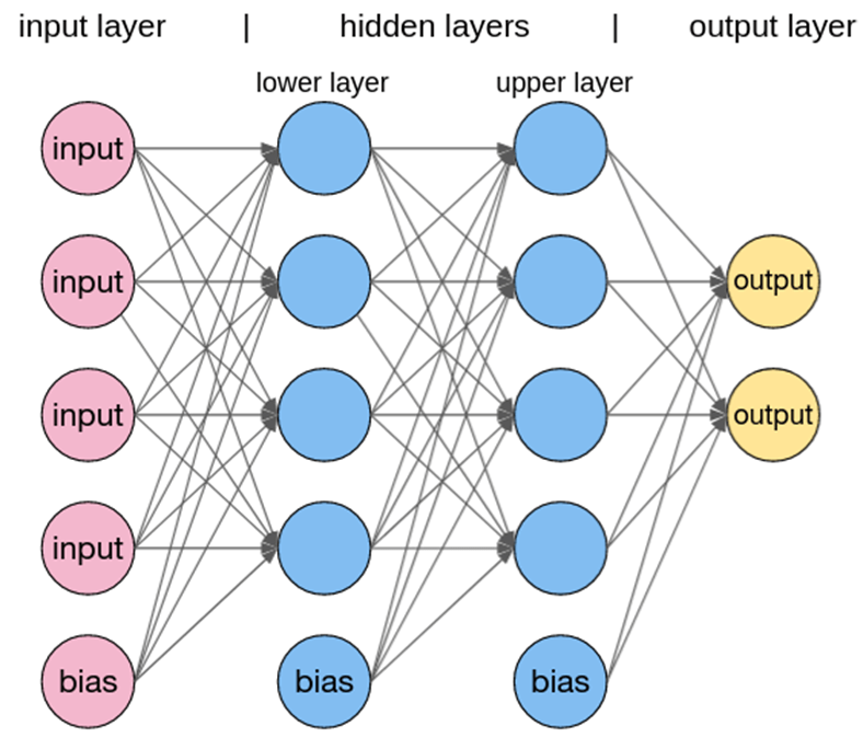
MLPs are the base of deep learning technology. It belongs to a class of feed-forward neural networks having various layers of perceptron’s. These perceptron’s have various activation functions in them. MLPs also have connected input and output layers and their number is the same. Also, mostly used to build image and speech recognition systems or some other types of the translation software.
The working of MLPs starts by feeding the data in the input data layer. The neurons present in the layer form a graph to establish a connection that passes in one direction. The weight of the input data is found to exist between the hidden layer and the input layer. MLPs use activation functions to determine which nodes are ready to fire. These activation functions include tanh function, sigmoid and ReLUs. MLPs are mainly used to train the models to understand what kind of correlation the layers are serving to achieve the desired output from the given data set. See the below image to understand better.
Restricted Boltzmann Machines
RBMs were developed by Geoffrey resemble stochastic neural networks that learn from the probability distribution in the given input set. This algorithm is mainly used in the field of dimension reduction, regression and classification, topic modelling and are considered the building blocks of Deep Belief Networks. RBIs consist of two layers namely the visible layer and the hidden layer. Both of these layers are connected through hidden units and have bias units connected to nodes that generate the output. Usually, RBMs have two phases namely forward pass and backward pass.
The functioning of RBMs is carries out by accepting inputs and translating them to numbers so that inputs are encoded in the forward pass. RBMs take into account the weight of every input, and the backward pass takes these input weights and translates them further into reconstructed inputs. Later, both of these translated inputs, along with individual weights, are combined. These inputs are then pushed to the visible layer where the activation is carries out, and output is generated that can be easily reconstructed. To understand this process, consider the below images.

Autoencoders
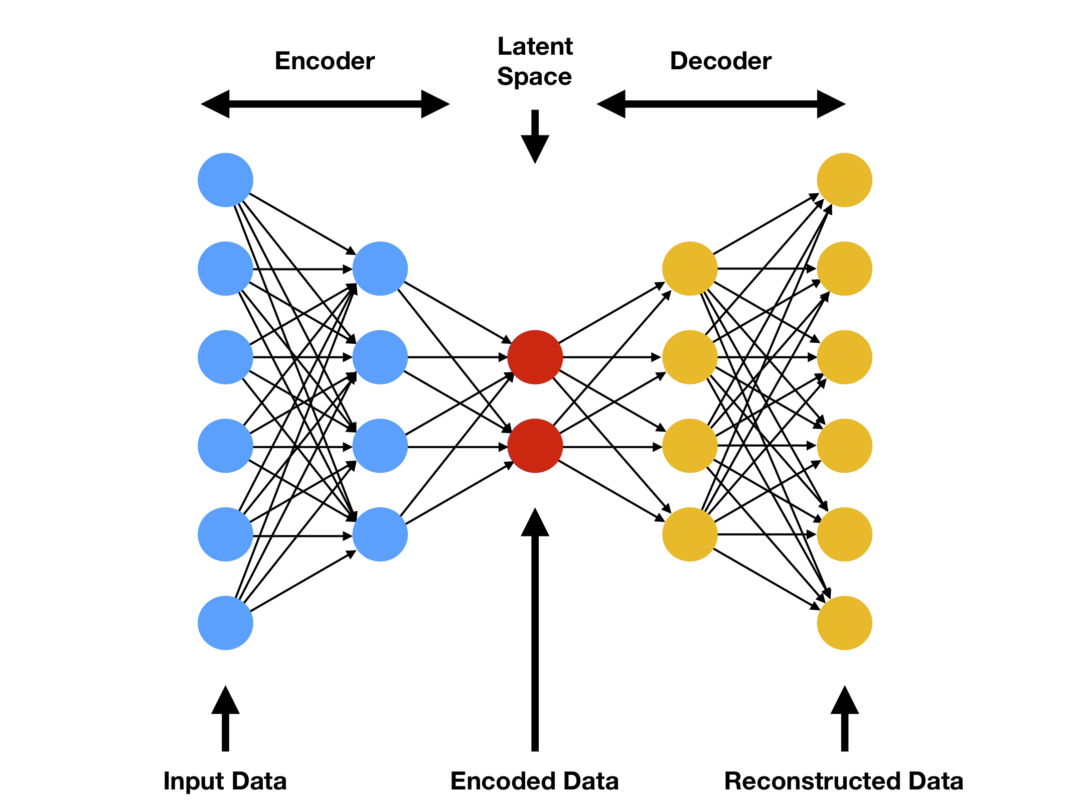
Autoencoders are a special type of neural network where inputs are outputs are found usually identical. It was designed to primarily solve the problems related to unsupervised learning. Autoencoders are highly trained neural networks that replicate the data. It is the reason why the input and output are generally the same. They are used to achieve task like pharma discovery, image processing, and population prediction.
Autoencoders constitute three components namely the encoder, the code, and the decoder. Autoencoders are built in such a structure that they can receive inputs are transform them into various representation. The attempts to copy the original input by reconstructing them is more accurate. They do this by encoding the image or input, reduce the size. If the image is not visible properly, they are passed to the neural network for clarification. Then, the clarified image is termed a reconstructed image and this resembles as accurate as of the previous image. To understand this complex process, see the below-provided image.