Denoising Images with Autoencoders Using TensorFlow and Python

Denoising Images with Autoencoders Using TensorFlow and Python

In today’s digital world, images play an important role in various applications, from medical imaging to self-driving cars. However, images are often corrupted by noise during transmission or storage, which can hinder the performance of image processing algorithms. In this blog post, we will explore how to use autoencoders to denoise images. We will implement this using Python and TensorFlow, a popular deep learning library.

Let’s begin by importing the necessary libraries and setting up our environment. The code snippet below does just that:

# Import libraries

from tensorflow.keras.datasets import mnist
from tensorflow.keras.layers import Conv2D, MaxPooling2D, UpSampling2D
from tensorflow.keras.models import Sequential
import numpy as np
import matplotlib.pyplot as plt

In this code, we import the MNIST dataset, which contains handwritten digits, and the required modules from TensorFlow and other libraries.

Loading and Preprocessing Data

Next, we load and preprocess the MNIST dataset. We convert the pixel values to a range between 0 and 1 and reshape the data to fit our model. Here’s how it’s done:

(x_train, _), (x_test, _) = mnist.load_data()

x_train = x_train.astype('float32') / 255.
x_test = x_test.astype('float32') / 255.
x_train = np.reshape(x_train, (len(x_train), 28, 28, 1))
x_test = np.reshape(x_test, (len(x_test), 28, 28, 1))

We also add some noise to our training and testing data to simulate real-world conditions:

noise_factor = 0.5
x_train_noisy = x_train + noise_factor * np.random.normal(loc=0.0, scale=1.0, size=x_train.shape)
x_test_noisy = x_test + noise_factor * np.random.normal(loc=0.0, scale=1.0, size=x_test.shape)

x_train_noisy = np.clip(x_train_noisy, 0., 1.)
x_test_noisy = np.clip(x_test_noisy, 0., 1.)

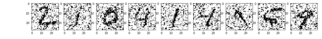
Visualizing Noisy Images

Let’s visualize some of the noisy images to understand the impact of noise:

plt.figure(figsize=(20, 2))
for i in range(1, 10):
    ax = plt.subplot(1, 10, i)
    plt.imshow(x_test_noisy[i].reshape(28, 28), cmap="binary")
plt.show()

This code snippet generates a plot of the noisy images.

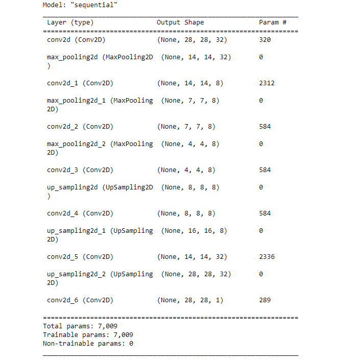
Building the Autoencoder Model

Now, we’ll construct our autoencoder model. An autoencoder is a neural network designed to encode input data into a lower-dimensional representation and then decode it to reconstruct the original data. Here’s our model architecture:

model = Sequential()
model.add(Conv2D(32, (3, 3), activation='relu', padding='same', input_shape=(28, 28, 1)))
model.add(MaxPooling2D((2, 2), padding='same'))
model.add(Conv2D(8, (3, 3), activation='relu', padding='same'))
model.add(MaxPooling2D((2, 2), padding='same'))
model.add(Conv2D(8, (3, 3), activation='relu', padding='same'))

model.add(MaxPooling2D((2, 2), padding='same'))

model.add(Conv2D(8, (3, 3), activation='relu', padding='same'))
model.add(UpSampling2D((2, 2)))
model.add(Conv2D(8, (3, 3), activation='relu', padding='same'))
model.add(UpSampling2D((2, 2)))
model.add(Conv2D(32, (3, 3), activation='relu'))
model.add(UpSampling2D((2, 2)))
model.add(Conv2D(1, (3, 3), activation='relu', padding='same'))

model.compile(optimizer='adam', loss='mean_squared_error')

model.summary()

In this model, we use convolutional layers for feature extraction and upsampling layers for reconstruction.

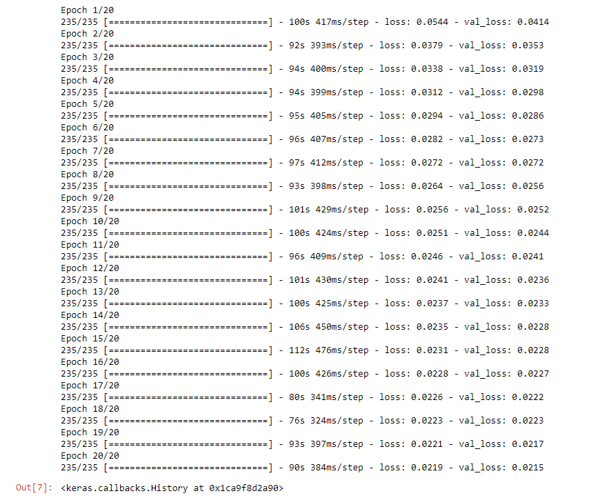
Training the Model

Now, it’s time to train our autoencoder:

model.fit(x_train_noisy, x_train, epochs=20, batch_size=256, shuffle=True, validation_data=(x_test_noisy, x_test))

In this code we trained the model for 20 epochs using the noisy training data. You can increase the number of epochs as per your need.

Evaluating the Model

After training, we can evaluate our model on the noisy test data:

model.evaluate(x_test_noisy, x_test)

This provides us with a measure of how well our model can denoise the images.

Saving the Model

If the model performs well, we can save it for future use:

model.save('denoising_mnist_autoencoder.model')

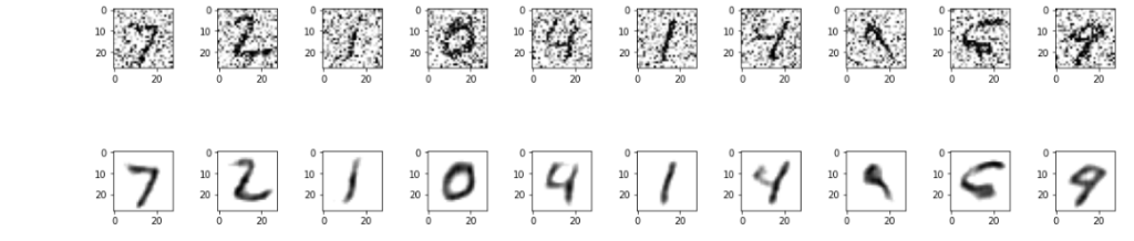
Visualizing Denoised Images

Finally, we can visualize the denoised images:

no_noise_img = model.predict(x_test_noisy)

plt.figure(figsize=(40, 4))
for i in range(10):
    ax = plt.subplot(3, 20, i + 1)
    plt.imshow(x_test_noisy[i].reshape(28, 28), cmap="binary")

    ax = plt.subplot(3, 20, 40 + i + 1)
    plt.imshow(no_noise_img[i].reshape(28, 28), cmap="binary")

plt.show()

This code generates a plot showing the original noisy images and their denoised counterparts.

Conclusion

In this blog post, we’ve explored how to use autoencoders to denoise images using Python and TensorFlow. By training an autoencoder on noisy images, we can remove unwanted artifacts and improve the quality of the reconstructed images. This technique has applications in various fields, including image processing and computer vision, where clean data is essential for accurate analysis and decision-making.

If you found this article helpful and insightful, I would greatly appreciate your support. You can show your appreciation by clicking on the button below. Thank you for taking the time to read this article

Nomidl

Denoising Images with Autoencoders Using TensorFlow and Python

Loading and Preprocessing Data

Visualizing Noisy Images

Building the Autoencoder Model

Training the Model

Evaluating the Model

Saving the Model

Visualizing Denoised Images

Conclusion

Popular Posts

Leave a Reply Cancel reply