Central Limit Theorem
We first need to introduce the normal (gaussian) distribution for central limit theorem to make sense. Normal distribution is a probability distribution that look like a bell.
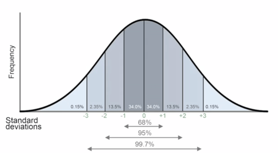
X-axis represents the values and y-axis represents the probability of observing these values. The sigma values represent standard deviation normal distribution is used to represent random variables with unknown distributions. The reason to justify why it can used to represent random variable with unknown distributions is the central limit theorem (CLT).
According to the CLT, as we take more samples from a distribution, the sample averages will tend towards a normal distribution regardless of the population distribution.
Consider a case that we need to learn the distribution of the heights of all 20-year-old people in a country. It is almost impossible and, of course not practical, to collect this data. So, we take samples of 20-years-old people across the country and calculate the average height of the people in samples. According to the CLT, as we take more samples from the population, sampling distribution will get close to normal distribution.
Why is it so important to have a normal distribution?
Normal distribution is described in terms of mean and standard deviation which can easily be calculated. And, if we know the mean and standard deviation of a normal distribution, we can compute pretty much everything about it.
P-Value
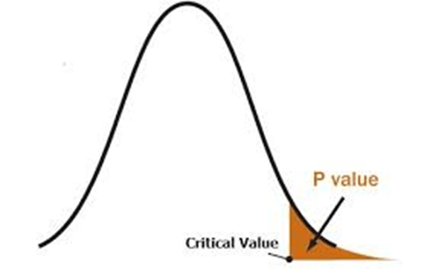
p-value is the probability of getting our observed value or values that have same or less chance to be observed. Consider the following probability distribution of a random variable A. it is highly likely to observe a value around 10. As the values get higher or lower, the probabilities decrease.
We have another random variable B and want to see if B is greater than A. the average sample means obtained from B is 12.5. the p value for 12.5 is the green area in the graph below. The green area indicates the probability of getting 12.5 or a more extreme value (higher than 12.5 in our case).
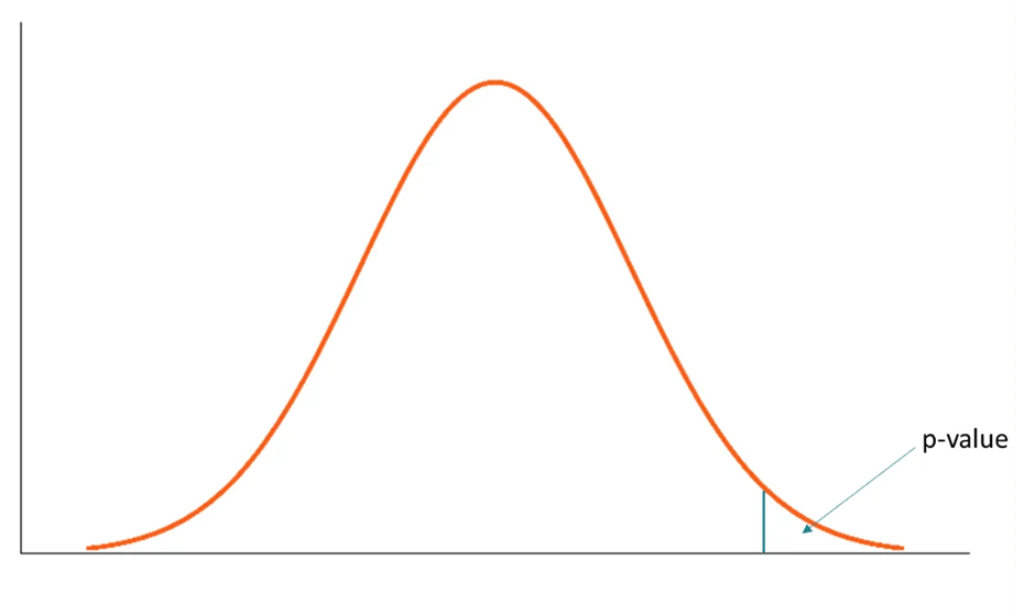
Let’s say the p value is 0.11 but how do we interpret it? A p value of 0.11 means that we are 89% sure of the results. In other words, there is 11% chance that the results are due to random chance. Similarly, a p value of 0.5 means that there is 5% chance that the results are due to random chance. If the average of sample means from the random variable B turns out to be 15 which is a more extreme value, the p value will be lower than 0.11.
Bias – Variance Trade off
Bias Occurs when we try to approximate a complex or complicated relationship with a much simpler model. Consider a case in which the relationship between independent variables (features) and dependent variables(target) is very complex and nonlinear. But, we try to build a model using linear regression. In this case, even if we have millions of training samples, we will not be able to build an accurate model. By using a simple model, we restrict the performance. The true relationship between the features and the target cannot be reflected. The models with high bias tend to underfit.
Variance occurs when the model is highly sensitive to the changes in the independent variables (features). The model tries to pick every detail about the relationship between features and target. It even learns the noise in the data which might randomly occur. A very small change in a feature might change the prediction of the model. Thus, we end up with a model that captures each and every detail on the training set will be very high. However, the accuracy of new, previously unseen samples will not be good because there will always be different variations in the features. This situation is also known as overfitting. The model overfits to the training data but fails to generalize well to that actual relationship within the dataset.
So, neither high bias nor high variance is good. The perfect model is the one with low bias and low variance. However, perfect models are challenging to find, if possible, at all. There is a trade-off between bias and variance.
Should aim to find the right balance between them. The key to success as a machine learning engineer is to master finding the right balance between bias and variance.
L1 and L2 Regularization
A solution to overfitting problem is to reduce the model complexity. Regularization controls the model complexity by penalizing higher terms in the model. If a regularization term is added, the model tries to minimize both loss and complexity of model.
L1 Regularization
L1 regularization forces the weights of uninformative features to be zero by subtracting a small from the weight at each iteration and thus making the weight zero, eventually.
L1 regularization penalizes |weight|
L2 Regularization
L2 regularization forces weights toward zero but it does not make them exactly zero. L2 regularization acts like a force that removes a small percentage of weights at each iteration. Therefore, weights will never be equal to zero.
L2 regularization penalizes (weight)2
Ridge regression used L2 regularization whereas Lasso regression used L1 regularization. Elastic net regression combines L1 and L2 regularization.
The curse of Dimensionality
In simplest terms, the curse of dimensionality indicates having too many features. More data is good but if it is well-structured. If we have many features (columns) but not enough observations (rows) to cope with, then we have a problem.
Having many features but not enough observations cause overfitting. The model, as expected, captures the details of the observations in the dataset rather than generalizing well to the relationship among features and target.
Another downside when we try to cluster the observations. Clustering algorithms use distance measures. Having too many features causes to have very similar distances between observations and thus making it very hard to group observations into clusters.
One solution for the curse of dimensionality would be to gather more observations (rows) by keeping the number of features the same. However, this would be time-consuming and not always be feasible. Furthermore, it will add an extra computation burden to the model. A better solution would be to use a dimensionality reduction algorithm such as PCA. Dimensionality reduction is reducing the number of features by deriving new features from the existing ones with an aim to preserve the variance in the dataset.