Are you curious about how machines can learn to understand and generate images? In this blog post, we’re going to delve into the fascinating world of Autoencoders using PyTorch, and we’ll explain this concept in simple terms. Autoencoders are a type of artificial neural network that can compress data and then reconstruct it. This article will guide you through the code that achieves this and even provide a glimpse of the results.
Understanding the Basics
Before we dive into the code, let’s understand the basics. An Autoencoder is a type of neural network that’s great at data compression. It can take complex data, like images, and represent them in a simpler form. The key idea is that Autoencoders learn to encode the data and then decode it back to its original form.
Now, let’s break down the provided code step by step.
First, we import essential libraries like PyTorch and torchvision, which help with deep learning and image processing. We also import modules for handling data and plotting graphs.
# Import necessary libraries and modules
import torch
import torchvision
import torch.nn as nn
import matplotlib.pyplot as plt
import numpy as np
from torchvision import transforms
Here, we set up a data transformation. We convert images from the MNIST dataset into tensors, a data format that’s easier for neural networks to work with.
# Define a data transformation to convert images to tensors
transform = transforms.ToTensor()
Loading the Data
We load the MNIST dataset, a collection of handwritten digits, which is commonly used for machine learning tasks. We have a training dataset and a validation dataset for testing.
# Load the MNIST dataset for training and validation
train_dataset = torchvision.datasets.MNIST(root='./data', train=True, download=True, transform=transform)
valid_dataset = torchvision.datasets.MNIST(root='./data', train=False, download=True, transform=transform)

# Create a data loader for training data with a batch size of 100
train_dl = torch.utils.data.DataLoader(train_dataset, batch_size=100)
Building the Encoder
# Define the Encoder class for the Variational Autoencoder (VAE)
class Encoder(nn.Module):
    def __init__(self, input_size=28 * 28, hidden_size1=128, hidden_size2=16, z_dim=2):
        super().__init__()
        self.fc1 = nn.Linear(input_size, hidden_size1)
        self.fc2 = nn.Linear(hidden_size1, hidden_size2)
        self.fc3 = nn.Linear(hidden_size2, z_dim)
        self.relu = nn.ReLU()

    def forward(self, x):
        x = self.relu(self.fc1(x))
        x = self.relu(self.fc2(x))
        x = self.fc3(x)
        return x
Building the Decoder
The Decoder does the opposite of the Encoder. It takes the compressed representation and generates an image.
# Define the Decoder class for the VAE
class Decoder(nn.Module):
    def __init__(self, output_size=28 * 28, hidden_size1=128, hidden_size2=16, z_dim=2):
        super().__init()
        self.fc1 = nn.Linear(z_dim, hidden_size2)
        self.fc2 = nn.Linear(hidden_size2, hidden_size1)
        self.fc3 = nn.Linear(hidden_size1, output_size)
        self.relu = nn.ReLU()

    def forward(self, x):
        x = self.relu(self.fc1(x))
        x = self.relu(self.fc2(x))
        x = torch.sigmoid(self.fc3(x))
        return x
Training the Model
We check if a GPU is available for faster computation. If not, we use the CPU.
# Check for GPU availability and set the device accordingly
device = torch.device('cuda' if torch.cuda.is_available() else 'cpu')
The encoder and decoder are initialized and placed on the selected device (GPU or CPU).
# Initialize the Encoder and Decoder on the selected device
enc = Encoder().to(device)
dec = Decoder().to(device)
Here, we set up the loss function, which measures the difference between the original image and the one generated by the decoder. We also prepare optimizers to update the encoder and decoder parameters.
# Define the loss function (Mean Squared Error) and the optimizers
loss_fn = nn.MSELoss()
optimizer_enc = torch.optim.Adam(enc.parameters())
optimizer_dec = torch.optim.Adam(dec.parameters())
Training the Model
# Store training loss values for each epoch
train_loss = []
num_epochs = 100
We keep track of the training loss for each epoch. The loss indicates how well the Autoencoder is learning to reconstruct images.
# Loop through training epochs
for epoch in range(num_epochs):
    train_epoch_loss = 0

    # Iterate through batches of training data
    for (imgs, _) in train_dl:
        imgs = imgs.to(device)
        imgs = imgs.flatten(1)
        latents = enc(imgs)
        output = dec(latents)
        loss = loss_fn(output, imgs)
        train_epoch_loss += loss.cpu().detach().numpy()
        optimizer_enc.zero_grad()
        optimizer_dec.zero_grad()
        loss.backward()
        optimizer_enc.step()
        optimizer_dec.step()

    train_loss.append(train_epoch_loss)
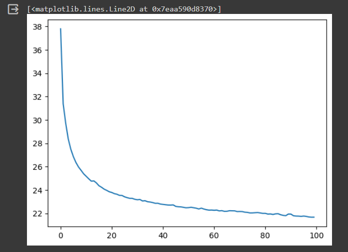
We create a plot to visualize how the training loss changes over the training epochs. This plot can help us see if the model is improving.
# Plot the training loss over epochs
plt.plot(train_loss)
We use the encoder to transform images into a simplified representation called latent space. We then save these representations and their corresponding labels for further analysis.
# Initialize variables to store latent representations and labels
values = None
all_labels = []

# Generate latent representations for the entire training dataset
with torch.no_grad():
    for (imgs, labels) in train_dl:
        imgs = imgs.to(device)
        imgs = imgs.flatten(1)
        all_labels.extend(list(labels.numpy())
        latents = enc(imgs)

        if values is None:
            values = latents.cpu()
        else:
            values = torch.vstack([values, latents.cpu()])
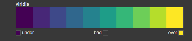
We set up a color map that we’ll use to visualize the latent space. This map helps us see patterns in the data.
# Create a color map for visualization
cmap = plt.get_cmap('viridis', 10)
We generate a scatter plot to visualize the latent space. Each point represents an image in the latent space, and the color represents the digit it corresponds to. This helps us see how the VAE has organized the data.
# Plot the scatter plot of latent space with color-coded labels
all_labels = np.array(all_labels)
values = values.numpy()
pc = plt.scatter(values[:, 0], values[:, 1], c=all_labels, cmap=cmap)
plt.colorbar(pc)

# Generate an image using a specific class's mean latent representation
with torch.no_grad():
    pred = dec(torch.Tensor(all_means[8])[None, ...].to(device)).cpu()
    transforms.ToPILImage()(pred.reshape(1, 28, 28))

Conclusion
In this blog post, we’ve explored the world of Autoencoders, a powerful concept in deep learning. We’ve seen how to build an Autoencoder in PyTorch, train it, and visualize its reconstruction capabilities.
Autoencoders are a fundamental concept in the field of machine learning and can be applied to various tasks, from image denoising to data compression. Understanding Autoencoders is a significant step towards grasping the potential of artificial intelligence and neural networks. We hope this article has made the concept of Autoencoders more accessible to you, and you’re now inspired to explore this exciting field further. Building and training neural networks like Autoencoders is a powerful skill, and you can use it to create intelligent systems that can analyze and generate data on their own.