VGG19 Image Recognition Model: Building a Classification

Building a Classification Model with VGG19 for Image Recognition

Image classification is a fascinating field of machine learning that involves teaching a computer to recognize and categorize objects or patterns within images. In this article, we will walk through the process of building a classification model using the VGG19 architecture for image recognition. We’ll start from importing the necessary libraries and proceed step by step, with clear explanations along the way.

Importing Libraries

We begin by importing the required libraries, which include popular tools for deep learning and data visualization:

import os
import cv2
import pickle
import numpy as np
import pandas as pd
import seaborn as sns
import matplotlib.pyplot as plt
import matplotlib.image as mpimg
import keras
import tensorflow
from tensorflow.keras.models import Model
from tensorflow.keras.utils import plot_model
from tensorflow.keras.models import Sequential
from tensorflow.keras.applications import VGG19
from tensorflow.keras.callbacks import EarlyStopping
from tensorflow.keras.preprocessing.image import ImageDataGenerator
from tensorflow.keras.layers import Input, Lambda, Dense, Flatten, Dropout, BatchNormalization, Activation
from sklearn metrics import confusion_matrix, classification_report, accuracy_score, recall_score, precision_score, f1_score

Defining Data Paths

Before diving into image processing, we need to specify the paths where our training, testing, and validation data is stored. These paths will point to directories containing image files.

train_path = r'path_to_training_data_directory'
test_path = r'path_to_testing_data_directory'
val_path = r'path_to_validation_data_directory'

Converting Images to Pixels

In the next step, we convert images into arrays of pixel values. This is essential because deep learning models work with numerical data.

def imagearray(path, size):
    data = []
    for folder in os.listdir(path):
        sub_path = path + "/" + folder
        for img in os.listdir(sub_path):
            image_path = sub_path + "/" + img
            img_arr = cv2.imread(image_path)
            img_arr = cv2.resize(img_arr, size)
            data.append(img_arr)
    return data

size = (250, 250)
train = imagearray(train_path, size)
test = imagearray(test_path, size)
val = imagearray(val_path, size)

Normalization

Normalization is crucial to ensure that all pixel values fall within the same range. In this case, we scale pixel values to a range of 0 to 1.

x_train = np.array(train)
x_test = np.array(test)
x_val = np.array(val)

x_train = x_train / 255.0
x_test = x_test / 255.0
x_val = x_val / 255.0

Defining Target Variables

Now, let’s define our target variables, which represent the classes of the images. We’ll use an ImageDataGenerator to create class labels for our data.

def data_class(data_path, size, class_mode):
    datagen = ImageDataGenerator(rescale=1./255)
    classes = datagen.flow_from_directory(data_path, target_size=size, batch_size=32, class_mode=class_mode)
    return classes

train_class = data_class(train_path, size, 'sparse')
test_class = data_class(test_path, size, 'sparse')
val_class = data_class(val_path, size, 'sparse')

y_train = train_class.classes
y_test = test_class.classes
y_val = val_class.classes

VGG19 Model

We will be using the VGG19 model, a powerful pre-trained neural network for image recognition tasks. We load this model and add a custom classification layer to the end.

vgg = VGG19(input_shape=(250, 250, 3), weights='imagenet', include_top=False)
for layer in vgg.layers:
    layer.trainable = False

x = Flatten()(vgg.output)
prediction = Dense(3, activation='softmax')(x)
model = Model(inputs=vgg.input, outputs=prediction)
model.compile(
  loss='sparse_categorical_crossentropy',
  optimizer="adam",
  metrics=['accuracy']
)

Model Training

We train our model using the training data and validate it on the validation data. We also incorporate early stopping to prevent overfitting.

early_stop = EarlyStopping(monitor='val_loss', mode='min', verbose=1, patience=5)
history = model.fit(x_train, y_train, validation_data=(x_val, y_val), epochs=10, callbacks=[early_stop], batch_size=30, shuffle=True)

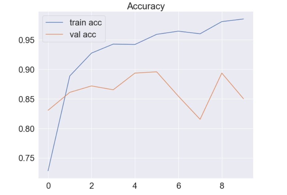
Visualization

We visualize the training and validation accuracy and loss over epochs using Matplotlib.

plt.figure(figsize=(10, 8))
plt.plot(history.history['accuracy'], label='train acc')
plt.plot(history.history['val_accuracy'], label='val acc')
plt.legend()
plt.title('Accuracy')
plt.show()

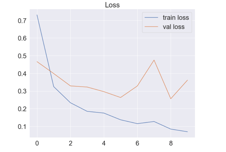
plt.figure(figsize=(10, 8))
plt.plot(history.history['loss'], label='train loss')
plt plot(history.history['val_loss'], label='val loss')
plt.legend()
plt.title('Loss')
plt.show()

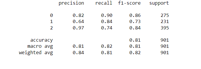
Model Evaluation

We evaluate the model’s performance on the test data and calculate key metrics like accuracy, precision, recall, and F1-score.

model.evaluate(x_test, y_test, batch_size=32)
y_pred = model.predict(x_test)
y_pred = np.argmax(y_pred, axis=1)
print(classification_report(y_pred, y_test))

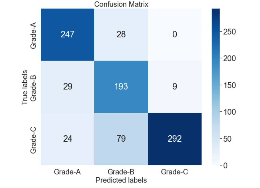
Confusion Matrix

A confusion matrix is a powerful tool for understanding model performance. We visualize it using Seaborn.

cm = confusion_matrix(y_pred, y_test)
plt.figure(figsize=(10, 8))
ax = plt.subplot()
sns.set(font_scale=2.0)
sns.heatmap(cm, annot=True, fmt='g', cmap="Blues", ax=ax)
ax.set_xlabel('Predicted labels', fontsize=20)
ax.set_ylabel('True labels', fontsize=20)
ax.set_title('Confusion Matrix', fontsize=20)
ax.xaxis.set_ticklabels(['Grade-A', 'Grade-B', 'Grade-C'], fontsize=20)
ax.yaxis.set_ticklabels(['Grade-A', 'Grade-B', 'Grade-C'], fontsize=20)

Saving the Model

After building and training our model, we save it for future use.

model.save("classification_model.h5")

Conclusion

In this article, we’ve walked through the process of building a classification model using the VGG19 architecture for image recognition. We’ve covered data preprocessing, model building, training, evaluation, and visualization. This is a powerful approach to recognize and classify images into different categories.

Spread the knowledge

Nomidl