Today we’re going to talk about how to manipulate images. These are preprocessing steps. When it comes to detecting edges and contours, noise plays a major role in the accuracy of the detection process. -The model needs to focus on the general details of their images in order to produce higher accuracies. -Blurring, thresholding, and morphological transformations are the techniques we use for this purpose.
Blurring
It can be tricky to negotiate which algorithms are used when performing noise reduction. It is important that you pay attention to these choices in order to get the best possible results.
If we make the images too blurry, then the data won’t show. We need an amount of blurring where we can maintain edges. in contrast to objects and still make the data show. We need a point of reference in order to sharpen our images later on.
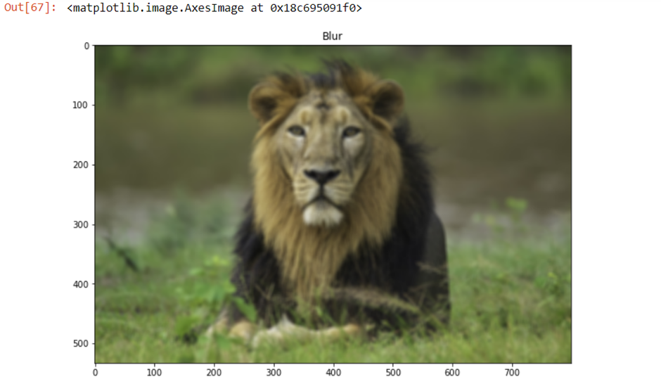
For OpenCV, there are four major techniques used to achieve blurring effects: Averaging blurring, Gaussian blurring, median blurring and bilateral filtering. For all four algorithms, the basic principle is using convolutional operations on the image. The value of each filter differs for those four different blurring methods. Average blurring method is the simplest and faster of all methods in-terms of computation time. The image is convolved with a Gaussian kernel of standard deviation equal to the pixel size around its center. Averaging blurring technique is about finding the average value for a set of pixels around the input point, then applying it to those pixels.
The average of the pixel values in a given kernel area will be used to replace a given value in the center. For example, let’s suppose we have a kernel with the size of 5X5. We calculate the average sin and put that on the center of the given area.
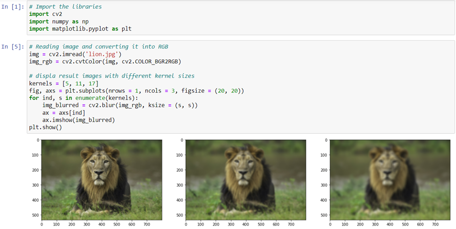
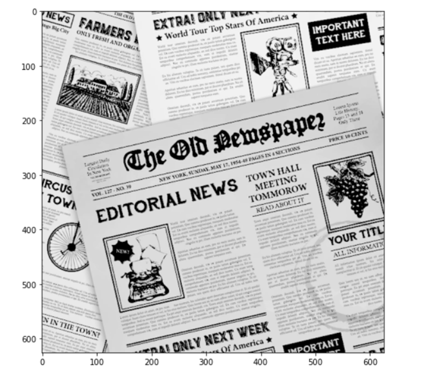
Then what will it be like if we increase the size of the kernel? As the size of filters gets bigger, pixel values will be normalized more. Therefore, we can expect images to get blurred more as well. Let’s check out the result with code below: (For comparison, I’ll keep attaching the original image to the result)
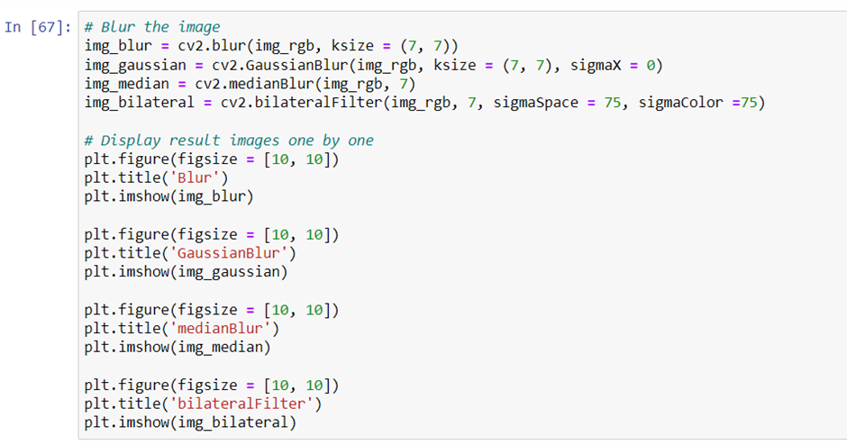
Medium blurring is the same as average blurring except that it uses the median value instead of the average. If a piece of content has sudden noises in the image, you should use medium blurring instead of average blurring.
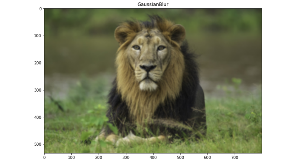
Gaussian blurring is a process in which input values are generated by a Gaussian function and requires a sigma value as its parameter. Applying this method to sounds with a normal distribution such as white noise would yield similar results.
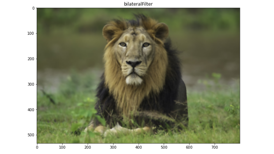
Bilateral Filtering is an advanced version of Gaussian blurring. Blurring produces not only vision graphics visuals but also removes noises and provides clean edges. The bilateral filter can also keep edges sharp while removing noise. Gaussian-distributed values are used, and both distance & pixel differences are taken into account. Therefore, it requires sigmaSpace and sigmaColor for the parameters.

Thresholding
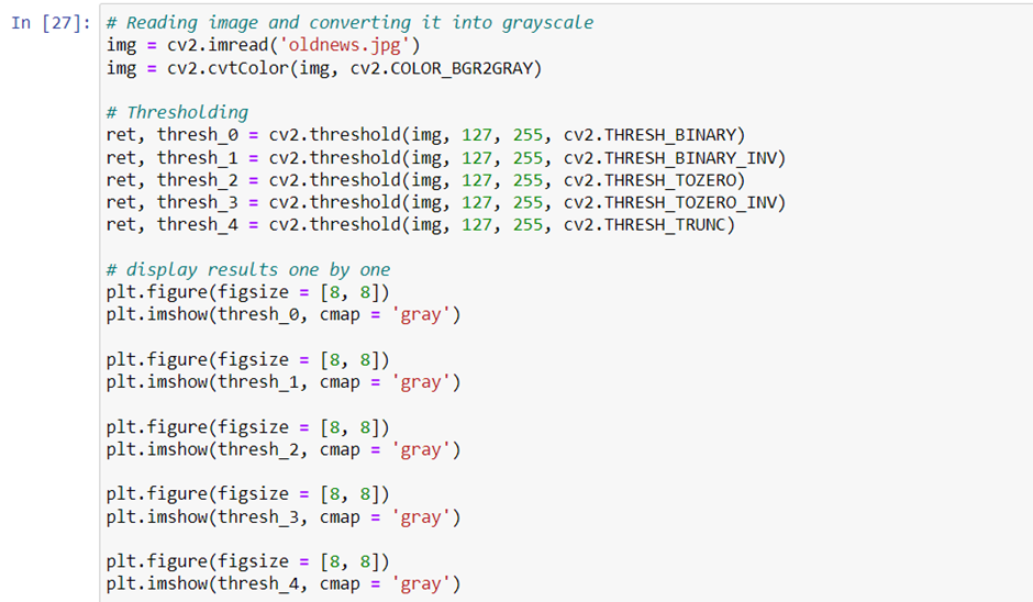
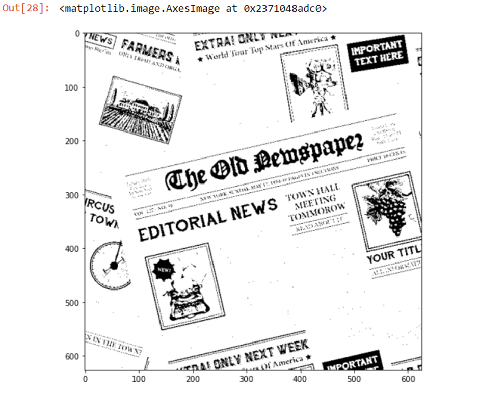
This algorithm allows you to convert images into binary images. It provides numerous settings that allow you to set desired threshold values and maximum pixel values before turning them into data.
There are five different types of thresholding: Binary, the inverse of Binary, Threshold to zero, the inverse of Threshold to Zero, and Threshold truncation.
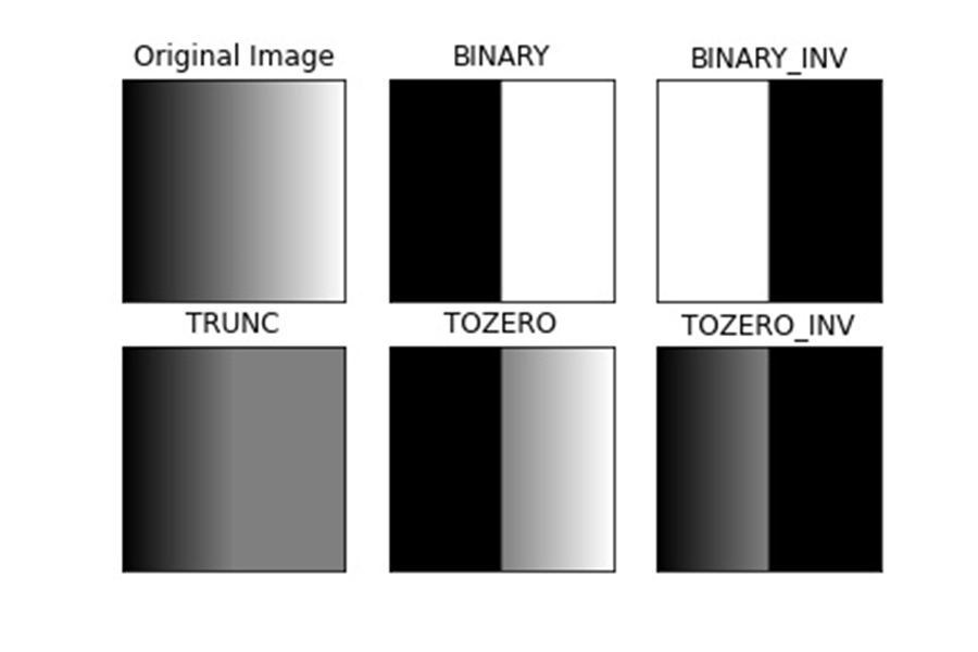
The intensity of every pixel in an image can be related to the amount of light it absorbs, or reflects, from the surrounding environment. This can be expressed mathematically and understood visually.
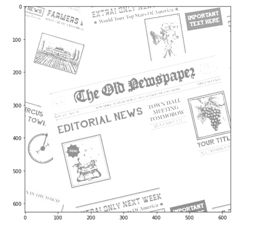
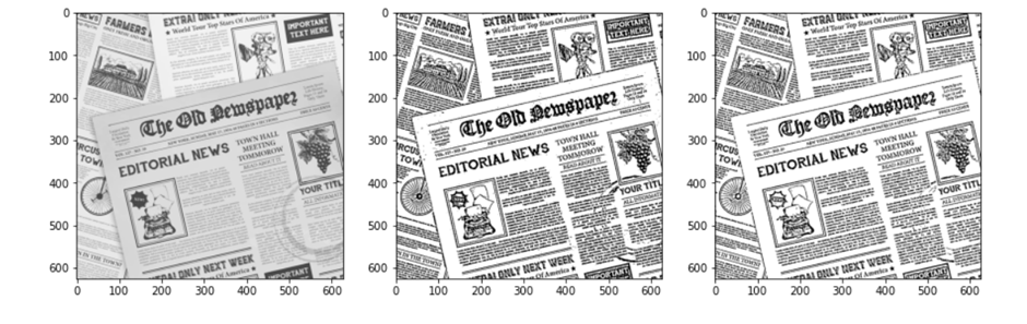
It’s a common misconception that you should use one algorithm for the whole image. In reality, it’s critical to apply each algorithm to a specific part of the photograph in order to ensure high quality results. Another approach would be to use different thresholds for each part of the image. There’s another technique called Adaptive Thresholding, which solves this issue by calculating the threshold within the neighborhood area of the image, we can achieve a better result from images with varying illumination.
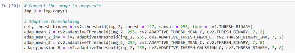
We need to convert the color image into grayscale to apply adaptive thresholding. The parameters of adaptive thresholding are maxvalue (which I set 255 above), adaptiveMethod , thresholdType , blockSize and C . And the adaptive method here has two kinds:
ADAPTIVE_THRESH_MEAN_C , ADAPTIVE_THRESH_GAUSSIAN_C.
Let’s just see how images are produced differently.

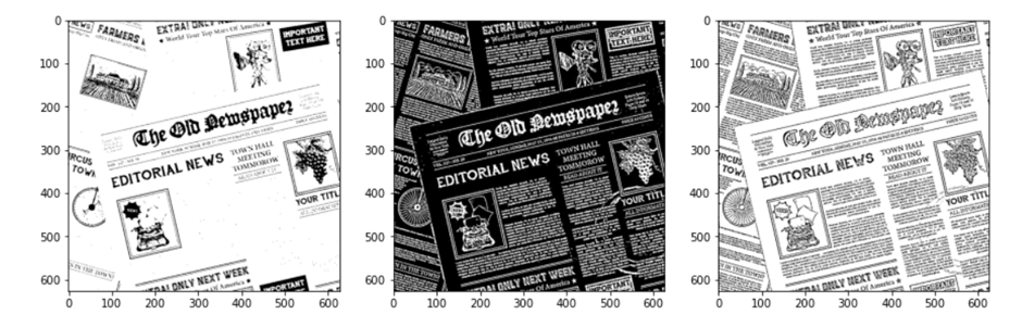
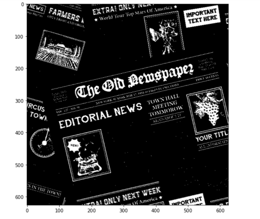
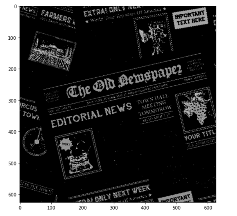
Gradient
Gradients can refer to all kinds of different things in mathematics. For example, a gradient is something that slopes away from some location. Gradients might be measured in terms of the steepness and general direction of the slope. As a function increases in power or height, the gradient will increase too. As it is a vector-valued function, it takes a direction and a magnitude as its components. Here we can also bring the same concept to the pixel values of colors in images as well. It’s an image gradient that can be used to point out directional changes in the intensity or color mode. You can use this concept for locating edges.
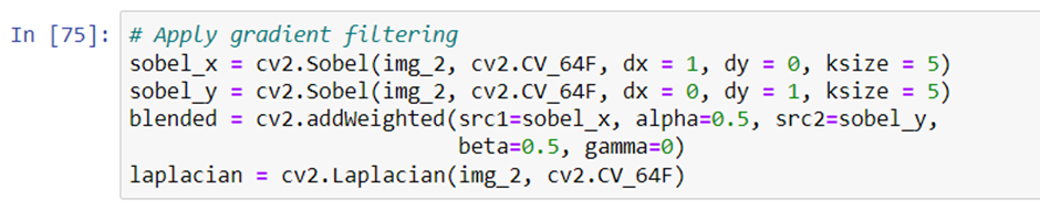
Sobel operation uses the Gaussian smoother along with differentiation. This function is applied to the data using cv2.Sobel(). There are two different directions to choose from, vertical and horizontal, and you have the option of choosing either or both of them (x and y). dx and dy indicate the derivatives. When dx = 1, it calculates the derivatives of the pixel values to make a filter.
Laplacian operation uses the second derivatives of x and y. The mathematical expression is shown below.
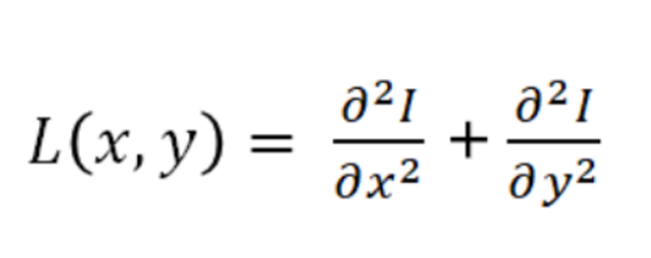
A picture is worth a thousand words. Let’s see how the images are like.
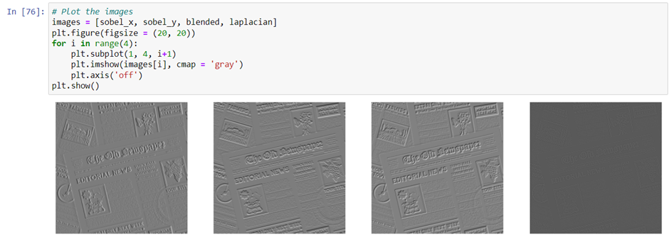
The first image has a clear pattern in the vertical direction. With the second image, we can see the horizontal edges. And both the third and fourth images, the edges on both directions are shown.
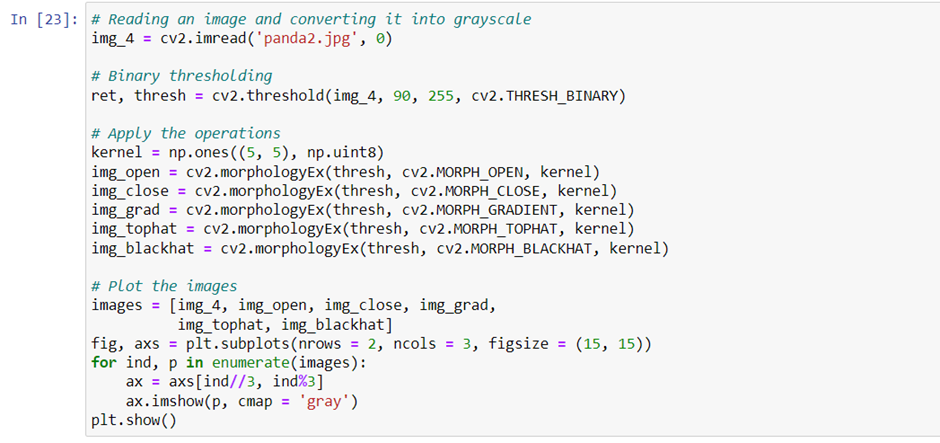
Morphological transformations
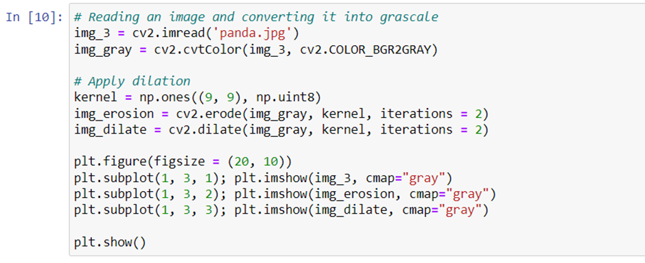
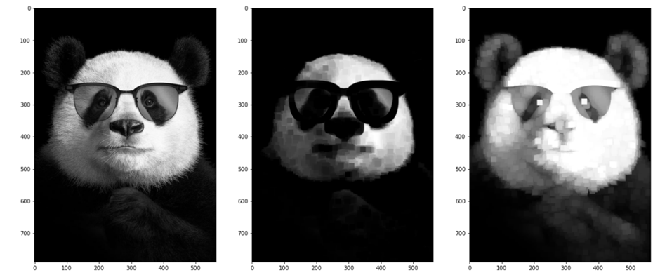
You can also manipulate the figures of images by filtering them, or called as morphological transformation. There are two types of morphological transformation you can perform: erosion and dilation. Let’s talk about the first one which is erosion.
The Erosion technique is a process that shrinks figures in an image by erasing some of the pixels in the underlying layer. Erosion can be processed in color or grey scale, depending on the size of the filters and the type of erosion being processed. The shape of these filters can be a rectangle, ellipse, or a cross shape.
Dilation is the opposite to erosion. It is making objects expand and the operation will be also opposite to that of erosion. Let’s check out the result with the code as follows.
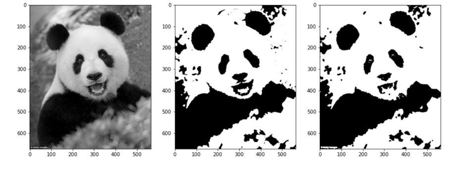
Opening and Closing operations are part of a procedure that is used to both erosion and dilation. Opening performs erosion first and then dilation is performed on the result from the erosion, while closing performs dilation first and the erosion on this result.
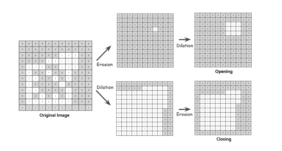
In this sketch, the figure was drawn with the edge of the rubber dipped in ink. Closing contours like this help to detect the overall shape of a figure, while opening contours such as these are useful to detect subpatterns. By implementing these operators with the function cv2.morphologyEx() shown below, we can make them easy to use. The parameter “op” indicates which type of operator we’re going to use.
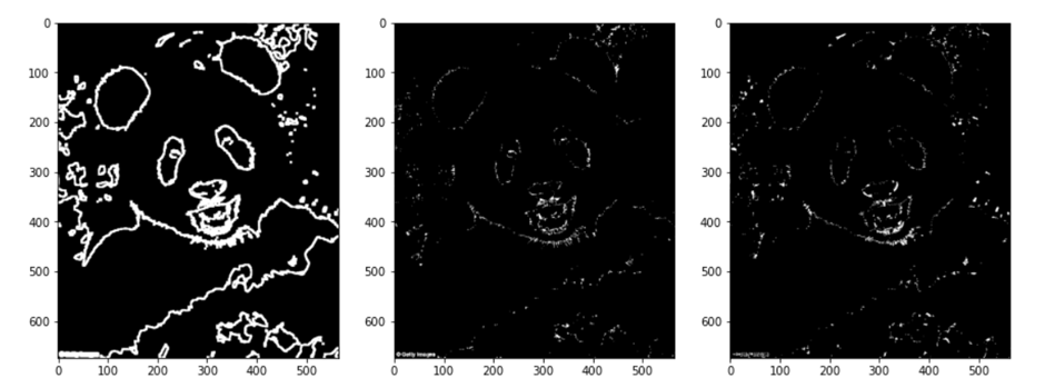
Gradient filter (MORPH_CGRADIENT) is the subtracted area from dilation to erosion. Top hat filter (MORPH_TOPHAT) is the subtracted area from opening to the original image while black hot filter (MORPH_BLACKHAT) is that from closing.
In this article we have discussed different types of blurring, thresholding and morphological techniques. In the next part we will be looking into the contours based techniques.