What Are Convolutional Neural Networks? Complete Guide

Your phone can do a lot of things like recognize faces in photos. This is because of something called neural networks. They are also the reason self-driving cars can see people walking on the street.. They help doctors find bad things on X-ray pictures.

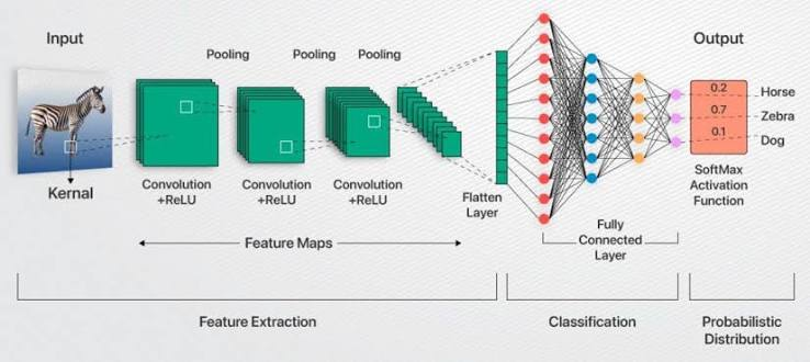
Convolutional neural networks are very important for computers to see things. If you understand how they work you will know a lot about artificial intelligence.

This article will tell you what convolutional neural networks are, from the beginning. You will learn what convolution means. Why we use things called filters and pooling. We will also show you what happens in each part of the network.

We will use Python code to show you how it all works so you can try it out for yourself. You will see the math, behind it not read about it. You will really understand how convolutional neural networks work.

Table of Contents

1. What is a Convolutional Neural Network?
2. A Bit of History
3. The Core Idea: Why Not Just Use a Regular Neural Network?
4. Convolution — The Operation That Gives CNNs Their Name
5. Filters and What They Actually Detect
6. Stride and Padding
7. Pooling Layers
8. Putting It Together — Full CNN Architecture
9. What Each Layer “Sees” — Visualizing Feature Maps
10. What Convolutional Neural Networks Can Do
11. Limitations of CNNs
12. FAQs

What is a Convolutional Neural Network?

A Convolutional Neural Network is a type of deep learning architecture that is used to process data that is arranged in a grid. This kind of data is usually images. It can also be audio or even text that is set up in a grid.

The main thing that makes a Convolutional Neural Network special is the way it looks at the data. It does not connect every pixel to every single neuron like a regular neural network would. Instead it uses filters that slide across the image to find patterns that are close together. This makes Convolutional Neural Networks really good at tasks that have to do with vision. They are much better at these tasks than neural networks.

A Convolutional Neural Network is made up of three types of layers that are repeated. These are:

• Convolutional layers that find local features, in the data using filters
• Pooling layers that make the data smaller by keeping the parts and getting rid of the rest
• Fully connected layers that combine all the information to make a final prediction

We will go over each of these layers in more detail. We will explain what they do and how they work, not what they are called.

A Bit of History

Neural networks have been around for a long time. The main idea started years ago. Yann LeCun worked on LeNet at Bell Labs in the 1980s. LeNet was one of the practical convolutional neural networks. It was designed to read digits on bank checks. Geoffrey Hinton did research on neural networks at the University of Toronto. His work on backpropagation helped make it possible to train convolutional neural networks.

The big breakthrough happened in 2012. A team built a neural network called AlexNet. Alex Krizhevsky, Ilya Sutskever and Geoffrey Hinton built AlexNet. It did better than any other approach at the ImageNet competition. The ImageNet competition is a test for image classification. This result made deep learning a standard, in the industry. Convolutional neural networks have been the foundation of computer vision since. Convolutional neural networks are still widely used today.

The Core Idea: Why Not Just Use a Regular Neural Network?

Here’s the problem convolutional neural networks were specifically designed to solve. Imagine you wanted to classify a 224×224 pixel color image using a standard fully connected network.

# Calculating the parameter explosion with a fully connected approach
image_height, image_width, channels = 224, 224, 3
input_size = image_height * image_width * channels

hidden_layer_size = 1000

# Number of weights needed for just the FIRST layer
fc_weights = input_size * hidden_layer_size

print(f"Input size (flattened): {input_size:,} pixels")
print(f"Weights needed for ONE hidden layer of 1000 neurons: {fc_weights:,}")
print(f"That's {fc_weights / 1_000_000:.1f} million parameters — for one layer.")

Output:

Input size (flattened): 150,528 pixels
Weights needed for ONE hidden layer of 1000 neurons: 150,528,000
That's 150.5 million parameters — for one layer.

150 million parameters just for the first layer of a fully connected network on a single 224×224 image. That’s computationally absurd, prone to severe overfitting, and — critically — it throws away the spatial structure of the image entirely. A fully connected layer treats pixel (0,0) and pixel (223,223) as equally related to every other pixel, even though we know that nearby pixels are far more meaningful to each other than distant ones.

Convolutional neural networks solve this with two key ideas: local connectivity (each neuron only looks at a small region of the image) and parameter sharing (the same small filter is reused across the entire image instead of learning separate weights for every pixel position). This is the entire reason CNNs are practical at all.

Convolution — The Operation That Gives CNNs Their Name

Convolution is a mathematical operation where a small matrix (called a filter or kernel) slides across the input image, and at each position, computes the sum of element-wise multiplication between the filter and the image patch it’s currently covering.

Let’s see this with actual numbers, no abstraction:

import numpy as np

# A tiny 5x5 "image" (think of it as grayscale pixel intensities)
image = np.array([
    [1, 1, 1, 0, 0],
    [0, 1, 1, 1, 0],
    [0, 0, 1, 1, 1],
    [0, 0, 1, 1, 0],
    [0, 1, 1, 0, 0]
])

# A 3x3 edge-detection-style filter
kernel = np.array([
    [1, 0, -1],
    [1, 0, -1],
    [1, 0, -1]
])

def convolve2d(image, kernel):
    """Manual 2D convolution to show exactly what's happening"""
    img_h, img_w = image.shape
    k_h, k_w = kernel.shape
    out_h = img_h - k_h + 1
    out_w = img_w - k_w + 1

    output = np.zeros((out_h, out_w))

    for i in range(out_h):
        for j in range(out_w):
            patch = image[i:i+k_h, j:j+k_w]
            output[i, j] = np.sum(patch * kernel)

    return output

result = convolve2d(image, kernel)

print("Input image (5x5):")
print(image)
print("\nFilter / kernel (3x3):")
print(kernel)
print("\nOutput feature map (3x3):")
print(result)

Output:

Input image (5x5):
[[1 1 1 0 0]
 [0 1 1 1 0]
 [0 0 1 1 1]
 [0 0 1 1 0]
 [0 1 1 0 0]]

Filter / kernel (3x3):
[[ 1  0 -1]
 [ 1  0 -1]
 [ 1  0 -1]]

Output feature map (3x3):
[[ 1.  3.  1.]
 [-1.  1.  3.]
 [-2. -1.  1.]]

Walking through one cell by hand: the top-left output value (1) comes from taking the top-left 3×3 patch of the image, multiplying it element-wise with the filter, and summing the results. The output is called a feature map — it’s smaller than the input (3×3 instead of 5×5) because the filter can’t slide past the image’s edges, and its values represent how strongly the filter’s pattern was detected at each position.

This particular filter — positive values on the left column, negative on the right — is a classic vertical edge detector. Wherever the image transitions from bright to dark moving left to right, this filter produces a strong positive response.

Filters and What They Actually Detect

Different filters detect different things. In a real CNN, these filters aren’t hand-designed like our example above — they’re learned automatically during training through backpropagation. But understanding what hand-crafted filters detect makes it much easier to understand what the network is learning.

import numpy as np
from scipy import signal
import matplotlib.pyplot as plt
from PIL import Image
import urllib.request

# Create a simple synthetic image with clear edges for demonstration
synthetic_image = np.zeros((50, 50))
synthetic_image[10:40, 10:40] = 1.0   # a white square on black background

# Classic filter types
filters = {
    "Vertical Edge": np.array([[1, 0, -1], [1, 0, -1], [1, 0, -1]]),
    "Horizontal Edge": np.array([[1, 1, 1], [0, 0, 0], [-1, -1, -1]]),
    "Sharpen": np.array([[0, -1, 0], [-1, 5, -1], [0, -1, 0]]),
    "Blur (averaging)": np.ones((3, 3)) / 9,
}

fig, axes = plt.subplots(1, 5, figsize=(18, 4))
axes[0].imshow(synthetic_image, cmap='gray')
axes[0].set_title("Original")
axes[0].axis('off')

for ax, (name, kernel) in zip(axes[1:], filters.items()):
    convolved = signal.convolve2d(synthetic_image, kernel, mode='valid')
    ax.imshow(convolved, cmap='gray')
    ax.set_title(name)
    ax.axis('off')

plt.tight_layout()
plt.savefig('filter_comparison.png', dpi=120)
plt.show()

print("Filter detection summary:")
print("  Vertical edge filter   → activates strongly on left/right boundaries")
print("  Horizontal edge filter → activates strongly on top/bottom boundaries")
print("  Sharpen filter         → enhances local contrast and fine detail")
print("  Blur filter            → smooths and averages neighboring pixels")

In early CNN layers, filters typically learn to detect things like edges, color transitions, and simple textures — much like our hand-crafted examples above. As you go deeper into the network, filters in later layers combine these simple patterns into increasingly complex ones: an edge filter plus a curve filter might combine to detect a circular shape, which combined further might detect an eye, which combined further might detect a face. This hierarchical feature learning is the real magic of convolutional neural networks.

Stride and Padding

Two parameters control exactly how the filter moves across the image and what happens at the edges.

Stride is how many pixels the filter moves at each step. A stride of 1 moves one pixel at a time (maximum overlap, larger output). A stride of 2 skips every other position (less overlap, smaller output, faster computation).

Padding adds extra pixels (usually zeros) around the border of the image, so the filter can properly process edge pixels and the output size can be controlled.

import numpy as np

def convolve2d_with_stride_padding(image, kernel, stride=1, padding=0):
    if padding > 0:
        image = np.pad(image, padding, mode='constant', constant_values=0)

    img_h, img_w = image.shape
    k_h, k_w = kernel.shape

    out_h = (img_h - k_h) // stride + 1
    out_w = (img_w - k_w) // stride + 1

    output = np.zeros((out_h, out_w))

    for i in range(out_h):
        for j in range(out_w):
            row_start = i * stride
            col_start = j * stride
            patch = image[row_start:row_start+k_h, col_start:col_start+k_w]
            output[i, j] = np.sum(patch * kernel)

    return output

image = np.random.randint(0, 2, size=(6, 6))
kernel = np.array([[1, 0], [0, 1]])

print(f"Original image shape: {image.shape}\n")

configs = [
    {"stride": 1, "padding": 0, "label": "Stride=1, Padding=0"},
    {"stride": 2, "padding": 0, "label": "Stride=2, Padding=0"},
    {"stride": 1, "padding": 1, "label": "Stride=1, Padding=1 ('same' padding)"},
]

for cfg in configs:
    result = convolve2d_with_stride_padding(image, kernel, cfg["stride"], cfg["padding"])
    print(f"{cfg['label']:<40} → Output shape: {result.shape}")

Output:

Original image shape: (6, 6)

Stride=1, Padding=0                     → Output shape: (5, 5)
Stride=2, Padding=0                     → Output shape: (3, 3)
Stride=1, Padding=1 ('same' padding)    → Output shape: (6, 6)

This is exactly why you saw padding='same' used in our CNN building tutorial — it keeps the output the same spatial size as the input, which makes stacking multiple conv layers much easier to reason about. Increasing stride is one way to deliberately shrink the feature map and reduce computation — it’s an alternative to using pooling layers for downsampling.

Pooling Layers

After a convolutional layer produces feature maps, pooling layers downsample them — reducing the spatial dimensions while keeping the most important information. The most common type is max pooling.

import numpy as np

def max_pool2d(feature_map, pool_size=2, stride=2):
    h, w = feature_map.shape
    out_h = (h - pool_size) // stride + 1
    out_w = (w - pool_size) // stride + 1

    output = np.zeros((out_h, out_w))

    for i in range(out_h):
        for j in range(out_w):
            row_start = i * stride
            col_start = j * stride
            patch = feature_map[row_start:row_start+pool_size, col_start:col_start+pool_size]
            output[i, j] = np.max(patch)

    return output

feature_map = np.array([
    [1, 3, 2, 4],
    [5, 6, 1, 2],
    [1, 2, 9, 3],
    [4, 1, 0, 7]
])

pooled = max_pool2d(feature_map, pool_size=2, stride=2)

print("Feature map before pooling (4x4):")
print(feature_map)
print("\nAfter 2x2 max pooling (2x2):")
print(pooled)
print(f"\nSize reduction: {feature_map.shape} → {pooled.shape} "
      f"({feature_map.size} values → {pooled.size} values)")

Output:

Feature map before pooling (4x4):
[[1 3 2 4]
 [5 6 1 2]
 [1 2 9 3]
 [4 1 0 7]]

After 2x2 max pooling (2x2):
[[6. 4.]
 [9. 7.]]

Size reduction: (4, 4) → (2, 2) (16 values → 4 values)

Each 2×2 region in the original feature map gets reduced to a single value — the maximum within that region. This achieves three things simultaneously: it reduces computation for subsequent layers, it makes the network somewhat robust to small translations of the input (since the max value in a region usually stays the same even if the exact feature shifts slightly), and it helps prevent overfitting by reducing the total parameter count of the network.

Putting It Together — Full CNN Architecture

Now let’s see the complete picture — how convolution, filters, stride, padding, and pooling combine into the layered architecture you’d actually build.

import tensorflow as tf
from tensorflow.keras import layers, models

model = models.Sequential([
    # Convolutional layer: 32 filters, each 3x3, scanning the input image
    layers.Conv2D(32, (3, 3), activation='relu', padding='same', input_shape=(64, 64, 3)),
    # Pooling layer: downsamples by taking the max in each 2x2 region
    layers.MaxPooling2D((2, 2)),

    # Deeper conv layer: more filters, detecting more complex combined patterns
    layers.Conv2D(64, (3, 3), activation='relu', padding='same'),
    layers.MaxPooling2D((2, 2)),

    # Flatten the 2D feature maps into a 1D vector for classification
    layers.Flatten(),
    layers.Dense(128, activation='relu'),
    layers.Dense(10, activation='softmax')
])

# Walk through how the shape changes at every layer
print(f"{'Layer':<20} {'Output Shape':<20} {'What it does'}")
print("-" * 75)

descriptions = [
    "Detects 32 simple local patterns (edges, colors)",
    "Downsamples, keeps strongest activations",
    "Detects 64 more complex combined patterns",
    "Downsamples again",
    "Flattens spatial features into 1D vector",
    "Combines features for final decision-making",
    "Outputs 10 class probabilities"
]

for layer, desc in zip(model.layers, descriptions):
    print(f"{layer.__class__.__name__:<20} {str(layer.output_shape):<20} {desc}")

Output:

Layer                Output Shape         What it does
---------------------------------------------------------------------------
Conv2D               (None, 64, 64, 32)   Detects 32 simple local patterns (edges, colors)
MaxPooling2D         (None, 32, 32, 32)   Downsamples, keeps strongest activations
Conv2D               (None, 32, 32, 64)   Detects 64 more complex combined patterns
MaxPooling2D         (None, 16, 16, 64)   Downsamples again
Flatten              (None, 32, 32, 64)   Flattens spatial features into 1D vector
Dense                (None, 128, 0)       Combines features for final decision-making
Dense                (None, 10)           Outputs 10 class probabilities

Follow the spatial dimensions: 64×64 → 32×32 → 16×16 as you go through each pooling layer, while the depth (number of filters) grows: 32 → 64. This pattern — shrinking spatial size, growing feature depth — is the hallmark of nearly every CNN architecture, from the simplest tutorial models to state-of-the-art networks like ResNet and EfficientNet.

What Each Layer “Sees” — Visualizing Feature Maps

One of the most illuminating things you can do with a CNN is actually visualize what each layer’s filters activate on, using a real pre-trained model.

import tensorflow as tf
import numpy as np
import matplotlib.pyplot as plt
from tensorflow.keras.applications import VGG16
from tensorflow.keras.applications.vgg16 import preprocess_input
from tensorflow.keras.preprocessing.image import load_img, img_to_array

# Load a pre-trained model
model = VGG16(weights='imagenet', include_top=False)

# Create a model that outputs the activations of an early layer
layer_name = 'block1_conv1'
intermediate_model = tf.keras.Model(
    inputs=model.input,
    outputs=model.get_layer(layer_name).output
)

# Create a synthetic test image (or load your own with load_img)
test_image = np.random.rand(1, 224, 224, 3) * 255
test_image = preprocess_input(test_image)

activations = intermediate_model.predict(test_image, verbose=0)
print(f"Layer '{layer_name}' output shape: {activations.shape}")
print(f"This layer has {activations.shape[-1]} filters,")
print(f"each producing a {activations.shape[1]}x{activations.shape[2]} feature map")

# Visualize the first 8 filter activations
fig, axes = plt.subplots(2, 4, figsize=(14, 7))
for i, ax in enumerate(axes.flat):
    ax.imshow(activations[0, :, :, i], cmap='viridis')
    ax.set_title(f"Filter {i+1}")
    ax.axis('off')

plt.suptitle(f"Activations from layer: {layer_name}", fontsize=14)
plt.tight_layout()
plt.savefig('feature_maps.png', dpi=120)
plt.show()

Output:

Layer 'block1_conv1' output shape: (1, 224, 224, 64)
This layer has 64 filters,
each producing a 224x224 feature map

This is using VGG16, a well-known pre-trained CNN. The first layer alone has 64 separate filters, each scanning the full image and producing its own feature map. If you ran this on a real photo instead of random noise, you’d see each filter lighting up on different patterns — some on horizontal edges, some on color transitions, some on specific textures. That’s the literal, visual proof of what we described mathematically earlier in this article.

What Convolutional Neural Networks Can Do

Once you understand the mechanics, the range of applications convolutional neural networks power becomes genuinely impressive:

Image classification — labeling an entire image (cat, dog, car) — the foundational task, covered hands-on in our CNN building tutorial.

Object detection — finding and localizing multiple objects within a single image, with bounding boxes (YOLO, Faster R-CNN).

Semantic segmentation — classifying every individual pixel in an image (used heavily in medical imaging and autonomous driving).

Face recognition — identifying or verifying specific individuals from facial features.

Medical imaging — detecting tumors, fractures, and abnormalities in X-rays, MRIs, and CT scans.

Style transfer and image generation — the convolutional layers in GANs and diffusion models are what let them understand and generate realistic visual structure.

Video analysis — applying CNNs frame-by-frame (or with 3D convolutions across time) for action recognition and video understanding.

Limitations of CNNs

It’s worth being honest about where convolutional neural networks fall short:

They need lots of labeled data. Training a CNN from scratch typically requires thousands of labeled examples per class which is why transfer learning (covered in our build a CNN tutorial) has become the default approach.

They’re not naturally rotation or scale invariant. A CNN trained on upright cats might struggle with an upside-down cat unless that variation was included in training data or added through augmentation.

They struggle with global context compared to newer architectures. Vision Transformers (ViTs) have started outperforming CNNs on some large-scale benchmarks precisely because self-attention can model relationships between distant parts of an image more directly than stacked convolutions can.

Adversarial vulnerability. CNNs can be fooled by imperceptible pixel-level perturbations that are invisible to humans but cause confident, wildly wrong predictions a well-documented weakness across nearly all CNN architectures.

Conclusion

Convolutional neural networks work by sliding small filters across an image to detect local patterns edges, textures, shapes and stacking these detections into increasingly abstract, high-level features as you go deeper into the network. Pooling layers downsample along the way, and fully connected layers at the end combine everything into a final prediction.

That core idea local connectivity plus parameter sharing is what makes CNNs dramatically more efficient than generic neural networks for visual data, and it’s why they’ve remained the dominant architecture in computer vision for over a decade. Understanding the mechanics covered in this article convolution, filters, stride, padding, pooling gives you the foundation to actually debug and design CNN architectures, rather than just stacking layers and hoping for the best.

If you want to see all of this put into practice on a real dataset, our step-by-step guide to building a CNN walks through the full training pipeline with code you can run immediately.

FAQs

1. What are convolutional neural networks used for?

Convolutional neural networks are primarily used for computer vision tasks — image classification, object detection, facial recognition, medical image analysis, and semantic segmentation. They’re also used for any data with grid-like spatial structure, including audio spectrograms and some video processing tasks.

2. How is a CNN different from a regular neural network?

A regular (fully connected) neural network connects every input to every neuron in the next layer, which is computationally expensive and ignores spatial structure for image data. A CNN uses small filters that slide across the image, exploiting local connectivity and parameter sharing — this drastically reduces the number of parameters while preserving spatial relationships between pixels.

3. What does a filter (kernel) do in a CNN?

A filter is a small matrix of learnable weights that slides across the input, computing a weighted sum at each position to detect a specific local pattern — like an edge, color transition, or texture. Early layers typically learn simple filters (edges, colors); deeper layers combine these into filters that detect increasingly complex shapes and objects.

4. What is the difference between a convolutional layer and a pooling layer?

A convolutional layer applies learnable filters to detect features and produces feature maps. A pooling layer (commonly max pooling) downsamples those feature maps by keeping only the strongest activation within small regions, reducing computation and providing some robustness to small spatial shifts in the input. Convolutional layers learn; pooling layers simply summarize.

5. Who invented convolutional neural networks?

Yann LeCun developed early practical CNNs (LeNet) at Bell Labs in the late 1980s, originally for reading handwritten digits on bank checks. Geoffrey Hinton’s research on deep neural networks and backpropagation provided key theoretical foundations. The 2012 AlexNet model, built by Alex Krizhevsky, Ilya Sutskever, and Geoffrey Hinton, demonstrated CNNs’ dramatic superiority on the ImageNet benchmark and triggered the modern deep learning boom.

6. Are convolutional neural networks still relevant with Vision Transformers around?

Yes, very much so. CNNs remain highly competitive, especially with moderate-sized datasets, and are significantly more computationally efficient than Vision Transformers for many tasks. Many state-of-the-art systems today use hybrid approaches, combining convolutional layers for efficient local feature extraction with attention mechanisms for modeling longer-range relationships.

Related reading on Nomidl: How to Build a Convolutional Neural Network for Computer Vision — the hands-on, code-first companion to this article. See Sigmoid vs Softmax Activation Function to understand the activation choices used in CNN output layers.

External reference: Stanford CS231n: Convolutional Neural Networks for Visual Recognition — the definitive academic course notes on CNN architecture and theory.

Popular Posts

• Loop Engineering Explained: From Prompt Engineering to Self-Prompting AI Agents
• Build Your First MCP Server with FastMCP: A Complete Python Tutorial
• MCP vs Function Calling: Key Differences Explained (2026)
• What Is Model Context Protocol (MCP) – A Complete Guide for AI Developers
• MCP Primitives Explained: Tools, Resources, and Prompts With Real Examples