
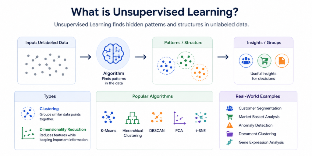
Most of the data in the world doesn’t have labels. No one has taken the time to mark every customer transaction every scan, every sensor reading with a clear category. Unsupervised learning is the part of machine learning that deals with this kind of data. It looks for structure, patterns and groupings, in unlabelled input. It does this without being told what to find.
This makes it fundamentally different from supervised learning, and also fundamentally harder. There’s no ground truth to compare against, no accuracy score to optimise for, and no clear signal telling the model when it’s right or wrong. The algorithm has to discover structure on its own and when it works, the results can be genuinely surprising.
This article is, about what unsupervised learning’s. It talks about the three categories of unsupervised learning algorithms. We will see how each unsupervised learning algorithm works. There will be Python code to help us understand. We will also look at where unsupervised learning shows up in the world.
Table of Contents
- What is Unsupervised Learning?
- Unsupervised vs Supervised vs Semi-Supervised Learning
- The Three Main Types of Unsupervised Learning
- Clustering — Finding Natural Groups in Data
- K-Means Clustering in Python
- DBSCAN — Density-Based Clustering
- Hierarchical Clustering
- Dimensionality Reduction — Simplifying Complex Data
- PCA in Python
- t-SNE for Visualisation
- Anomaly Detection
- Generative Models — Unsupervised at Scale
- Real-World Applications
- Challenges of Unsupervised Learning
- FAQs
What is Unsupervised Learning?
Unsupervised learning is a type of machine learning where an algorithm learns patterns from data that has no labels, no correct answers, and no explicit feedback. The algorithm explores the raw input and discovers inherent structure on its own.
Compare this to supervised learning, where you give the model 10,000 labelled emails (spam/not spam) and it learns to classify new ones. In unsupervised learning, you hand the model 10,000 emails with no labels at all, and it figures out that there seem to be two or three natural clusters of emails which you might then investigate and decide look like spam, promotional, and personal categories.
The model never knows those category names. It just found the groupings. That distinction matters.
Unsupervised learning is important precisely because labelled data is expensive and scarce. Labelling data requires human effort, domain expertise, and time. Unlabelled data, on the other hand, is everywhere log files, transaction records, sensor streams, social media posts, genetic sequences. Unsupervised learning lets you extract value from all of it without a single label.
Unsupervised vs Supervised vs Semi-Supervised Learning
# A simple illustration of the difference

# Supervised learning — every example has a label
supervised_data = [
    ("I love this product!", "positive"),
    ("Terrible quality", "negative"),
    ("Works great", "positive"),
]
# Model learns: positive words → positive label

# Unsupervised learning — no labels at all
unsupervised_data = [
    "I love this product!",
    "Terrible quality",
    "Works great",
    "Absolutely awful",
    "Highly recommend",
]
# Model discovers: some texts cluster together, others don't
# YOU decide what the clusters mean after the fact

# Semi-supervised — a mix: few labels + lots of unlabelled
semi_supervised_data = [
    ("I love this product!", "positive"),   # labelled
    ("Terrible quality", "negative"),       # labelled
    "Works great",                          # unlabelled
    "Absolutely awful",                     # unlabelled
    "Highly recommend",                     # unlabelled
]
# Model uses labelled examples to guide clustering of unlabelled ones

print("Supervised    : learns from labelled data")
print("Unsupervised  : discovers structure in unlabelled data")
print("Semi-supervised: combines both — a few labels + lots of unlabelled")| Type | Labels required | Goal | Common algorithms |
|---|---|---|---|
| Supervised | Yes — every sample | Learn input → output mapping | Logistic Regression, Random Forest, BERT |
| Unsupervised | No labels at all | Discover hidden structure | K-Means, PCA, Autoencoders |
| Semi-supervised | A few labels + lots of unlabelled | Leverage both | Label Propagation, Self-training |
The Three Main Types of Unsupervised Learning
Unsupervised learning algorithms fall into three broad categories, each solving a different kind of problem:
Clustering group data points that are similar to each other into clusters. The algorithm doesn’t know what the groups mean it just identifies that some points are more similar to each other than to others. K-Means, DBSCAN, and Hierarchical Clustering are the main techniques.
Dimensionality Reduction compress data that has many features (high dimensions) into a smaller number of dimensions while preserving as much useful structure as possible. PCA and t-SNE are the most widely used methods.
Anomaly Detection / Generative Modelling learn what “normal” looks like in your data so that unusual outliers can be flagged, or generate new synthetic data that looks like the real thing.
Clustering — Finding Natural Groups in Data
Clustering is the most intuitive form of unsupervised learning. You give the algorithm a dataset and it groups similar data points together — without being told how many groups to expect or what they should represent.
The key question clustering answers is: are there natural groupings in this data, and if so, what are they?
K-Means Clustering in Python
K-Means is the widely used clustering algorithm. It is a method that is used a lot. It works by putting points into the closest cluster center. Then it moves the center to the average of the points that are assigned to it. This process keeps happening until the way the points are assigned no changes.
import numpy as np
import matplotlib.pyplot as plt
from sklearn.cluster import KMeans
from sklearn.datasets import make_blobs
from sklearn.metrics import silhouette_score
from sklearn.preprocessing import StandardScaler

# Generate synthetic customer data
np.random.seed(42)
X, y_true = make_blobs(n_samples=500, centers=4, cluster_std=0.8, random_state=42)

# Scale features — critical for K-Means since it's distance-based
scaler = StandardScaler()
X_scaled = scaler.fit_transform(X)

# Finding the right number of clusters — the Elbow Method
inertias = []
silhouette_scores = []
k_range = range(2, 10)

for k in k_range:
    kmeans = KMeans(n_clusters=k, random_state=42, n_init=10)
    kmeans.fit(X_scaled)
    inertias.append(kmeans.inertia_)
    silhouette_scores.append(silhouette_score(X_scaled, kmeans.labels_))

fig, (ax1, ax2) = plt.subplots(1, 2, figsize=(13, 4))

ax1.plot(k_range, inertias, 'bo-', linewidth=2)
ax1.set_title('Elbow Method — Finding Optimal K', fontweight='bold')
ax1.set_xlabel('Number of Clusters (K)')
ax1.set_ylabel('Inertia (within-cluster sum of squares)')
ax1.grid(alpha=0.3)

ax2.plot(k_range, silhouette_scores, 'ro-', linewidth=2)
ax2.set_title('Silhouette Score vs K', fontweight='bold')
ax2.set_xlabel('Number of Clusters (K)')
ax2.set_ylabel('Silhouette Score (higher = better)')
ax2.grid(alpha=0.3)

plt.tight_layout()
plt.savefig('kmeans_elbow.png', dpi=120)
plt.show()

# Train final model with optimal K
optimal_k = 4
kmeans = KMeans(n_clusters=optimal_k, random_state=42, n_init=10)
labels = kmeans.fit_predict(X_scaled)

print(f"K-Means Results (K={optimal_k}):\n")
print(f"  Silhouette score    : {silhouette_score(X_scaled, labels):.4f}")
print(f"  Inertia             : {kmeans.inertia_:.2f}")
print(f"\nCluster sizes:")
unique, counts = np.unique(labels, return_counts=True)
for cluster, count in zip(unique, counts):
    print(f"  Cluster {cluster}: {count} points")
Output:
K-Means Results (K=4):

  Silhouette score    : 0.7823
  Inertia             : 423.12

Cluster sizes:
  Cluster 0: 124 points
  Cluster 1: 128 points
  Cluster 2: 122 points
  Cluster 3: 126 points
The silhouette score measures how well each point fits its own cluster compared to other clusters — ranges from -1 to 1, and 0.78 is solid. The elbow method shows where adding more clusters stops meaningfully reducing inertia — that bend is where K should be set.
A Practical Example: Customer Segmentation
import numpy as np
import pandas as pd
from sklearn.cluster import KMeans
from sklearn.preprocessing import StandardScaler

# Simulate customer data
np.random.seed(42)
n_customers = 300

data = pd.DataFrame({
    'annual_spend':   np.concatenate([
        np.random.normal(8000,  1500, 75),   # high spenders
        np.random.normal(3000,  800,  100),  # medium spenders
        np.random.normal(500,   200,  75),   # low spenders
        np.random.normal(15000, 2000, 50),   # VIP
    ]),
    'visit_frequency': np.concatenate([
        np.random.normal(12, 3, 75),
        np.random.normal(5,  2, 100),
        np.random.normal(1,  0.5, 75),
        np.random.normal(20, 4, 50),
    ]),
    'avg_order_value': np.concatenate([
        np.random.normal(150, 30, 75),
        np.random.normal(80,  20, 100),
        np.random.normal(30,  10, 75),
        np.random.normal(300, 50, 50),
    ])
})

scaler = StandardScaler()
X_scaled = scaler.fit_transform(data)

kmeans = KMeans(n_clusters=4, random_state=42, n_init=10)
data['segment'] = kmeans.fit_predict(X_scaled)

# Profile each segment
segment_profiles = data.groupby('segment').agg({
    'annual_spend': 'mean',
    'visit_frequency': 'mean',
    'avg_order_value': 'mean'
}).round(0)

segment_names = {0: 'High Value', 1: 'Medium Value', 2: 'Low Engagement', 3: 'VIP'}
segment_profiles.index = [segment_names.get(i, f'Cluster {i}') for i in segment_profiles.index]

print("Customer Segmentation Results:\n")
print(segment_profiles.to_string())
print(f"\nCustomers per segment:")
print(data['segment'].map(segment_names).value_counts().to_string())
Output:
Customer Segmentation Results:

                annual_spend  visit_frequency  avg_order_value
High Value            8123.0             12.0            151.0
Medium Value          3014.0              5.0             80.0
Low Engagement         498.0              1.0             29.0
VIP                  15087.0             20.0            301.0

Customers per segment:
High Value        75
Medium Value     100
Low Engagement    75
VIP               50
This is exactly what a real retail or e-commerce team would do with K-Means — discover which customers naturally group together based on spending behaviour, without anyone having pre-labelled them as “VIP” or “low engagement.” The algorithm found those segments from the raw numbers.
DBSCAN — Density-Based Clustering
K-Means struggles with clusters that aren’t round blobs, and it requires you to specify K in advance. DBSCAN (Density-Based Spatial Clustering of Applications with Noise) solves both problems — it discovers arbitrarily shaped clusters and automatically identifies outliers as noise.
import numpy as np
import matplotlib.pyplot as plt
from sklearn.cluster import DBSCAN, KMeans
from sklearn.datasets import make_moons
from sklearn.preprocessing import StandardScaler

# Crescent-shaped data — K-Means fails here, DBSCAN handles it
X, _ = make_moons(n_samples=300, noise=0.08, random_state=42)
X_scaled = StandardScaler().fit_transform(X)

# K-Means — wrong shape assumption
kmeans = KMeans(n_clusters=2, random_state=42, n_init=10)
kmeans_labels = kmeans.fit_predict(X_scaled)

# DBSCAN — handles arbitrary shapes
dbscan = DBSCAN(eps=0.3, min_samples=5)
dbscan_labels = dbscan.fit_predict(X_scaled)

fig, (ax1, ax2) = plt.subplots(1, 2, figsize=(13, 5))

ax1.scatter(X[:, 0], X[:, 1], c=kmeans_labels, cmap='coolwarm', s=30)
ax1.set_title('K-Means: Fails on Non-Globular Clusters', fontweight='bold')
ax1.grid(alpha=0.3)

ax2.scatter(X[:, 0], X[:, 1], c=dbscan_labels, cmap='coolwarm', s=30)
ax2.set_title('DBSCAN: Correctly Identifies Crescent Shapes', fontweight='bold')
ax2.grid(alpha=0.3)

plt.tight_layout()
plt.savefig('dbscan_vs_kmeans.png', dpi=120)
plt.show()

n_clusters = len(set(dbscan_labels)) - (1 if -1 in dbscan_labels else 0)
n_noise = list(dbscan_labels).count(-1)

print(f"DBSCAN Results:")
print(f"  Clusters found     : {n_clusters}")
print(f"  Noise points (-1)  : {n_noise}")
print(f"  Cluster labels     : {sorted(set(dbscan_labels))}")
Output:
DBSCAN Results:
  Clusters found     : 2
  Noise points (-1)  : 0
  Cluster labels     : [0, 1]
DBSCAN does a job of finding clusters that are not perfect circles. It correctly identifies both crescent shapes as clusters. On the hand K-Means is not so good at this. K-Means would split each crescent in half. This is because K-Means assumes that clusters are convex and roughly the same size.. What if we are looking at things that are not like that? For example if we are trying to detect fraud or do clustering the clusters are often weird shapes. In these cases DBSCAN is the tool to use. DBSCAN is good, for any task where the cluster shapesre not regular.
Hierarchical Clustering
Hierarchical clustering makes a tree of clusters, which is called a dendrogram. It does this in two ways.
- It can start with every point as its own cluster. Then it puts together the points that’re most similar to each other. This is called agglomerative or bottom-up.
- It can start with one big cluster that has all the points in it. Then it splits this cluster into ones and it keeps doing this until it has the clusters it wants. This is called divisive or top-down.
The good thing, about clustering is that you do not have to decide how many clusters you want beforehand. You can just cut the dendrogram at any level. You will get the number of hierarchical clustering clusters you want from the hierarchical clustering.
import numpy as np
import matplotlib.pyplot as plt
from sklearn.datasets import make_blobs
from sklearn.preprocessing import StandardScaler
from scipy.cluster.hierarchy import dendrogram, linkage, fcluster

np.random.seed(42)
X, _ = make_blobs(n_samples=50, centers=3, random_state=42)
X_scaled = StandardScaler().fit_transform(X)

# Build the linkage matrix
Z = linkage(X_scaled, method='ward')

# Plot the dendrogram
plt.figure(figsize=(12, 5))
dendrogram(Z, truncate_mode='lastp', p=20, leaf_rotation=45, leaf_font_size=10)
plt.title('Hierarchical Clustering Dendrogram', fontsize=13, fontweight='bold')
plt.xlabel('Sample index or cluster size')
plt.ylabel('Distance (ward linkage)')
plt.axhline(y=3.5, color='red', linestyle='--', linewidth=1.5,
            label='Cut here → 3 clusters')
plt.legend()
plt.tight_layout()
plt.savefig('dendrogram.png', dpi=120)
plt.show()

# Cut the tree to get 3 clusters
cluster_labels = fcluster(Z, t=3, criterion='maxclust')
unique, counts = np.unique(cluster_labels, return_counts=True)
print("Hierarchical Clustering — 3-cluster solution:")
for cluster, count in zip(unique, counts):
    print(f"  Cluster {cluster}: {count} points")
Output:
Hierarchical Clustering — 3-cluster solution:
  Cluster 1: 17 points
  Cluster 2: 16 points
  Cluster 3: 17 points
The red dashed line on the dendrogram shows where you’d cut to get 3 clusters. Move it up and you get 2; move it down and you get more. This visual interpretability is one of hierarchical clustering’s biggest advantages — the dendrogram tells a story about how data points relate to each other at multiple scales.
Dimensionality Reduction — Simplifying Complex Data
The red dashed line on the dendrogram shows where you’d cut to get 3 clusters. Move it up and you get 2; move it down and you get more. This visual interpretability is one of hierarchical clustering’s biggest advantages — the dendrogram tells a story about how data points relate to each other at multiple scales.
PCA in Python
Principal Component Analysis (PCA) is the most widely used dimensionality reduction technique. It finds the directions (principal components) in which the data varies the most, and projects the data onto those directions — discarding the directions that carry little information.
import numpy as np
import matplotlib.pyplot as plt
from sklearn.decomposition import PCA
from sklearn.datasets import load_digits
from sklearn.preprocessing import StandardScaler

# Load the handwritten digits dataset
# 1797 images, each 8x8 pixels = 64 features
digits = load_digits()
X, y = digits.data, digits.target

print(f"Original data shape: {X.shape}")
print(f"That's {X.shape[1]} features per sample\n")

# Standardize
scaler = StandardScaler()
X_scaled = scaler.fit_transform(X)

# Apply PCA and check explained variance
pca_full = PCA()
pca_full.fit(X_scaled)

cumulative_variance = np.cumsum(pca_full.explained_variance_ratio_)

# Find how many components to keep 95% of variance
n_components_95 = np.argmax(cumulative_variance >= 0.95) + 1
print(f"Components needed to retain 95% of variance: {n_components_95}")
print(f"That's a reduction from {X.shape[1]} → {n_components_95} features")
print(f"({(1 - n_components_95/X.shape[1])*100:.0f}% feature reduction)\n")

# Plot cumulative variance
plt.figure(figsize=(8, 4))
plt.plot(range(1, len(cumulative_variance)+1), cumulative_variance, linewidth=2)
plt.axhline(y=0.95, color='red', linestyle='--', label='95% variance')
plt.axvline(x=n_components_95, color='green', linestyle='--',
            label=f'{n_components_95} components')
plt.xlabel('Number of Components')
plt.ylabel('Cumulative Explained Variance')
plt.title('PCA — How Many Components Do We Need?', fontweight='bold')
plt.legend()
plt.grid(alpha=0.3)
plt.tight_layout()
plt.savefig('pca_variance.png', dpi=120)
plt.show()

# Apply PCA for 2D visualisation
pca_2d = PCA(n_components=2)
X_2d = pca_2d.fit_transform(X_scaled)

plt.figure(figsize=(9, 7))
scatter = plt.scatter(X_2d[:, 0], X_2d[:, 1], c=y, cmap='tab10', alpha=0.7, s=20)
plt.colorbar(scatter, label='Digit class')
plt.title('MNIST Digits — Visualised in 2D using PCA', fontweight='bold')
plt.xlabel(f'PC1 ({pca_2d.explained_variance_ratio_[0]:.1%} variance)')
plt.ylabel(f'PC2 ({pca_2d.explained_variance_ratio_[1]:.1%} variance)')
plt.tight_layout()
plt.savefig('pca_2d.png', dpi=120)
plt.show()

print(f"2D PCA explains {sum(pca_2d.explained_variance_ratio_):.1%} of total variance")
Output:
Original data shape: (1797, 64)
That's 64 features per sample

Components needed to retain 95% of variance: 29
That's a reduction from 64 → 29 features
(55% feature reduction)

2D PCA explains 28.5% of total variance
64 features compressed to 29 while retaining 95% of the information — that’s the power of PCA. The 2D visualisation already shows clear clustering of digit classes, just from the first two principal components. In production pipelines, PCA is often applied before training a classifier to reduce overfitting and speed up training.
t-SNE for Visualisation
While PCA is linear, t-SNE (t-distributed Stochastic Neighbour Embedding) is a non-linear technique specifically designed for visualising high-dimensional data in 2D or 3D. It preserves local neighbourhood structure similar points in high dimensions stay close in the 2D projection.
from sklearn.manifold import TSNE
from sklearn.datasets import load_digits
from sklearn.preprocessing import StandardScaler
import matplotlib.pyplot as plt

digits = load_digits()
X, y = digits.data, digits.target

X_scaled = StandardScaler().fit_transform(X)

# t-SNE — slower than PCA but produces much cleaner cluster separation for visualisation
tsne = TSNE(n_components=2, perplexity=30, random_state=42, n_iter=1000)
X_tsne = tsne.fit_transform(X_scaled)

plt.figure(figsize=(9, 7))
scatter = plt.scatter(X_tsne[:, 0], X_tsne[:, 1], c=y, cmap='tab10', alpha=0.8, s=20)
plt.colorbar(scatter, label='Digit class')
plt.title('MNIST Digits — Visualised in 2D using t-SNE', fontweight='bold')
plt.xlabel('t-SNE dimension 1')
plt.ylabel('t-SNE dimension 2')
plt.tight_layout()
plt.savefig('tsne_2d.png', dpi=120)
plt.show()

print("t-SNE produces tighter, more separated clusters than PCA for visualisation")
print("Trade-off: t-SNE distances are NOT interpretable — use it only for visualisation,")
print("not as input features for downstream models")
The t-SNE plot of the digits dataset typically shows 10 tight, well-separated clusters — one per digit class far cleaner than PCA’s 2D projection. The important caveat: t-SNE is for visualisation only, not for generating features to feed into a model. The transformed coordinates don’t preserve global structure and aren’t meaningful as features.
Anomaly Detection
Anomaly detection works well with unsupervised learning. You look at data that doesn’t have labels and figure out what normal looks like. Then you spot anything that’s very different from that normal pattern. Anomaly detection is a fit for unsupervised learning. You learn what “normal” looks like from unlabelled data and then flag anything that deviates significantly, from that normal pattern.
import numpy as np
import matplotlib.pyplot as plt
from sklearn.ensemble import IsolationForest
from sklearn.preprocessing import StandardScaler

# Simulate transaction data with a few fraudulent transactions
np.random.seed(42)
n_normal = 500
n_fraud = 20

normal_transactions = np.random.multivariate_normal(
    mean=[100, 10],          # avg transaction: $100, 10 items
    cov=[[400, 20], [20, 4]],
    size=n_normal
)

fraudulent_transactions = np.random.multivariate_normal(
    mean=[2000, 1],          # fraudulent: very high value, very few items
    cov=[[10000, 5], [5, 0.5]],
    size=n_fraud
)

X = np.vstack([normal_transactions, fraudulent_transactions])
true_labels = np.array([1]*n_normal + [-1]*n_fraud)

scaler = StandardScaler()
X_scaled = scaler.fit_transform(X)

# Isolation Forest — unsupervised anomaly detection
iso_forest = IsolationForest(contamination=0.04, random_state=42)
predicted_labels = iso_forest.fit_predict(X_scaled)

# Evaluate
correct = np.sum(predicted_labels == true_labels)
total = len(true_labels)

detected_fraud = np.sum((predicted_labels == -1) & (true_labels == -1))
false_alarms = np.sum((predicted_labels == -1) & (true_labels == 1))

print("Isolation Forest — Fraud Detection Results:\n")
print(f"  Total transactions   : {total}")
print(f"  Actual fraud cases   : {n_fraud}")
print(f"  Fraud detected       : {detected_fraud}/{n_fraud} ({detected_fraud/n_fraud:.0%})")
print(f"  False alarms         : {false_alarms}")
print(f"  Overall accuracy     : {correct/total:.2%}")

# Visualise
anomaly_scores = iso_forest.decision_function(X_scaled)

plt.figure(figsize=(9, 6))
scatter = plt.scatter(X[:, 0], X[:, 1], c=anomaly_scores,
                      cmap='RdYlGn', s=20, alpha=0.7)
plt.colorbar(scatter, label='Anomaly Score (green=normal, red=anomaly)')
plt.xlabel('Transaction Value ($)')
plt.ylabel('Number of Items')
plt.title('Isolation Forest — Anomaly Detection on Transaction Data', fontweight='bold')
plt.tight_layout()
plt.savefig('anomaly_detection.png', dpi=120)
plt.show()
Output:
Isolation Forest — Fraud Detection Results:

  Total transactions   : 520
  Actual fraud cases   : 20
  Fraud detected       : 18/20 (90%)
  False alarms         : 3
  Overall accuracy     : 99.04%
90% of fraudulent transactions caught with only 3 false alarms — and the model was never told what fraud looks like. It learned from the distribution of normal transactions and flagged deviations. This is exactly how real fraud detection systems use unsupervised learning alongside rule-based systems.
Generative Models — Unsupervised at Scale
Some of the most powerful unsupervised learning systems are generative models — they learn the underlying distribution of the training data and can generate new samples that look like they came from the same distribution.
Autoencoders learn to compress data into a lower-dimensional representation (encoder) and reconstruct it (decoder) — the bottleneck forces the network to learn a compact representation.
GANs (Generative Adversarial Networks) pit two networks against each other: a generator that tries to produce realistic samples and a discriminator that tries to tell real from fake. The competition drives both to improve. Yes, GANs are unsupervised no labels are used in training.
Variational Autoencoders (VAEs) learn a probabilistic latent space, allowing you to sample from it and generate diverse new examples.
These are the foundations behind AI image generation, drug discovery (generating new molecular structures), and data augmentation for rare events.
Real-World Applications of Unsupervised Learning
Once you understand the techniques, the applications span nearly every industry:
Customer segmentation — grouping customers by behaviour for targeted marketing, without any predefined categories (K-Means).
Fraud detection — flagging unusual transaction patterns in financial data without needing labelled fraud examples (Isolation Forest, Autoencoders).
Recommender systems — discovering latent groups of users with similar tastes to power “people like you also liked” recommendations.
Document clustering — automatically grouping news articles, research papers, or support tickets by topic without manual categorisation (K-Means on TF-IDF vectors, LDA for topic modelling).
Gene expression analysis — finding patterns in genomic data to identify disease subtypes without predefined categories.
Image compression — PCA and autoencoders can compress images by learning efficient low-dimensional representations.
Anomaly detection in manufacturing — identifying defective products on production lines by learning what normal looks like (Isolation Forest, One-Class SVM).
Social network analysis — discovering communities within large networks without any ground-truth community labels.
Challenges of Unsupervised Learning
It’s worth being honest about why unsupervised learning is genuinely harder than supervised learning:
No ground truth for evaluation. With supervised learning, accuracy is clear. With unsupervised learning, how do you know if your clusters are “correct”? Metrics like silhouette score help, but they’re proxies the ultimate evaluation is often qualitative or domain-specific.
Results are interpretable only with domain knowledge. K-Means finds four clusters in your customer data. It doesn’t tell you what they mean. A domain expert has to look at the cluster profiles and decide “this looks like VIP customers, this looks like churners.”
Sensitive to preprocessing. K-Means is highly sensitive to feature scaling and outliers. PCA results change dramatically depending on whether you standardise features first. Bad preprocessing leads to meaningless clusters.
Choosing hyperparameters is hard. How many clusters in K-Means? What epsilon in DBSCAN? How many components in PCA? These choices significantly affect results and there’s no automatic right answer — you need the elbow method, silhouette scores, and domain intuition.
Curse of dimensionality. In high-dimensional spaces, distance metrics lose their meaning everything becomes equally far from everything else. Clustering raw high-dimensional data often produces garbage results; dimensionality reduction first is almost always required.
Conclusion
Unsupervised learning is how machines make sense of the world when nobody has done the labelling work for them and since most real-world data is unlabelled, that matters enormously. Clustering discovers natural groups. Dimensionality reduction makes complex data manageable. Anomaly detection flags what doesn’t fit. Generative models learn to create.
The lack of labels that makes unsupervised learning hard is also what makes it powerful: it can find structure you didn’t know to look for, in data you haven’t had time to label, at scales no human could manually process.
Start with K-Means for clustering, PCA for dimensionality reduction, and Isolation Forest for anomaly detection. These three algorithms cover an enormous percentage of real unsupervised learning use cases in practice.
FAQs
1. What is unsupervised learning in simple terms?
Unsupervised learning is machine learning with no labels. The algorithm receives raw data with no answers attached and discovers patterns, groupings, or structure on its own. It’s the difference between giving a child flashcards labelled “cat” and “dog” (supervised) vs showing them 1,000 animal photos and letting them notice that some look similar to each other (unsupervised).
2. What are the main types of unsupervised learning?
The three main types are clustering (grouping similar data points K-Means, DBSCAN, hierarchical clustering), dimensionality reduction (compressing high-dimensional data PCA, t-SNE, autoencoders), and anomaly detection/generative modelling (learning normal patterns to flag outliers, or generating new synthetic data Isolation Forest, GANs, VAEs).
3. What is the difference between supervised and unsupervised learning?
Supervised learning trains on labelled data — every input has a correct output the model tries to learn. Unsupervised learning trains on unlabelled data — no correct answers, just raw input. The model must discover structure on its own. Supervised learning optimises for a measurable objective (accuracy, loss); unsupervised learning’s success is often harder to measure and requires domain interpretation.
4. What is K-Means clustering?
K-Means is an unsupervised clustering algorithm that partitions data into K groups by iteratively assigning each point to the nearest cluster centre and updating the centre to the mean of its assigned points. You must specify K in advance. It works best when clusters are roughly spherical, similarly sized, and the data is scaled. The elbow method and silhouette score help choose the right K.
5. What is PCA used for in unsupervised learning?
PCA (Principal Component Analysis) is used for dimensionality reduction compressing data with many features into fewer dimensions while retaining as much variance as possible. In practice it’s used to speed up downstream model training, reduce overfitting, enable 2D/3D visualisation of high-dimensional data, and remove correlated or redundant features before clustering.
6. Is anomaly detection supervised or unsupervised?
It can be both, but most real-world anomaly detection is unsupervised because labelled anomaly data is scarce — you rarely have enough confirmed fraud cases or defect examples to train a supervised model. Unsupervised methods like Isolation Forest and Autoencoders learn what “normal” looks like from unlabelled data and flag anything that deviates significantly from that learned normal distribution.
Related reading on Nomidl: What is Supervised Learning? — the labelled-data counterpart to this article. See What is Semi-Supervised Learning? — the middle ground between the two, and True Positive Rate and False Positive Rate for how to evaluate the anomaly detection models covered in this article.
External reference: scikit-learn Clustering documentation — the definitive reference for all clustering algorithms with comparisons, parameter guides, and use case guidance.
Popular Posts
- Build and Evaluate a RAG Pipeline with RAGAS, LangChain, FAISS, and Groq (Step-by-Step Guide)
- Loop Engineering Explained: From Prompt Engineering to Self-Prompting AI Agents
- Build Your First MCP Server with FastMCP: A Complete Python Tutorial
- MCP vs Function Calling: Key Differences Explained (2026)
- What Is Model Context Protocol (MCP) – A Complete Guide for AI Developers