
Pick the wrong one between sigmoid vs softmax activation function for your output layer, and your model’s predictions will be mathematically wrong even if your architecture, data, and training process are all perfect. This is one of those deep learning decisions that looks like a minor detail but actually breaks things silently if you get it wrong.
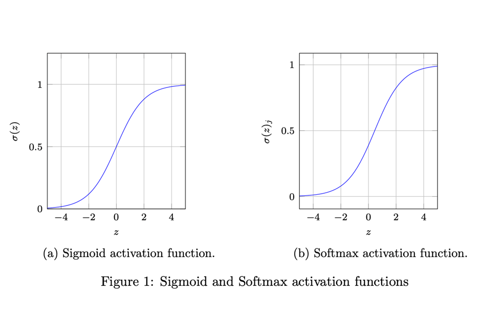
Both functions squash raw numbers into probability-like values between 0 and 1. But they answer fundamentally different questions. Sigmoid answers “what’s the probability of this one thing being true?” Softmax answers “given several possible classes, which one is most likely, and how confident are we relative to the others?”
This article will breaks down exactly how each function works mathematically, shows the code, plots the curves, and tells you precisely when to use which.
Table of Contents
- Quick Answer
- What is the Sigmoid Activation Function?
- What is the Softmax Activation Function?
- The Math: Sigmoid vs Softmax Side by Side
- Visualizing Both Functions
- Sigmoid vs Softmax: Full Comparison Table
- Code Walkthrough: Sigmoid and Softmax from Scratch
- Using Sigmoid and Softmax in Real Models
- The Multi-Label Trap — Where People Get This Wrong
- Which Loss Function Pairs with Which
- FAQs
Quick Answer
Before the deep dive, here’s the one-line version:
Sigmoid outputs an independent probability between 0 and 1 for a single class — use it for binary classification or multi-label classification (where multiple labels can be true at once).
Softmax outputs a probability distribution across multiple classes that always sums to exactly 1 — use it for multi-class classification (where exactly one class is correct).
That single distinction independent probabilities vs a joint distribution that sums to 1 is the difference between sigmoid vs softmax activation function in a nutshell. Everything else in this article expands on why that matters.
What is the Sigmoid Activation Function?
The sigmoid function squashes any real number into a range between 0 and 1. It’s defined as:
σ(x) = 1 / (1 + e^(-x))Feed it a large positive number, you get something close to 1. Feed it a large negative number, you get something close to 0. Feed it 0, you get exactly 0.5.
Key properties:
- Output range:
(0, 1)— never quite reaches the endpoints - S-shaped curve, smooth and differentiable everywhere
- Each output is computed independently of other outputs
- Outputs for different classes do not need to sum to 1
That last point is the one people often miss. If you apply sigmoid to 3 different output neurons, you might get 0.9, 0.85, and 0.3 — these don’t need to add up to anything in particular. Each is its own independent yes/no probability.
import numpy as np

def sigmoid(x):
    return 1 / (1 + np.exp(-x))

# Example: binary classification — "is this email spam?"
logits = np.array([-3, -1, 0, 1, 3])
probabilities = sigmoid(logits)

print(f"{'Logit':>8} {'Sigmoid Output':>16}")
print("-" * 26)
for logit, prob in zip(logits, probabilities):
    print(f"{logit:>8} {prob:>16.4f}")
Output:
   Logit   Sigmoid Output
--------------------------
      -3           0.0474
      -1           0.2689
       0           0.5000
       1           0.7311
       3           0.9526
A logit of 0 gives exactly 0.5 — perfectly uncertain. As the logit moves positive, the probability climbs toward 1. As it moves negative, it drops toward 0.
What is the Softmax Activation Function?
The softmax function takes a vector of raw scores (logits) for multiple classes and converts them into a probability distribution where every value is between 0 and 1, and all values sum to exactly 1. It’s defined as:
softmax(x_i) = e^(x_i) / Σ e^(x_j) for j = 1 to nIn words: take the exponential of each value, then divide by the sum of all the exponentials. This forces the outputs to compete with each other — if one class’s probability goes up, the others must go down, because the total has to stay at 1.
import numpy as np

def softmax(x):
    exp_x = np.exp(x - np.max(x))  # subtract max for numerical stability
    return exp_x / np.sum(exp_x)

# Example: multi-class classification — "which animal is in this image?"
logits = np.array([2.0, 1.0, 0.1, -1.0])
class_names = ["cat", "dog", "bird", "fish"]

probabilities = softmax(logits)

print(f"{'Class':<8} {'Logit':>8} {'Softmax Probability':>22}")
print("-" * 40)
for cls, logit, prob in zip(class_names, logits, probabilities):
    print(f"{cls:<8} {logit:>8.1f} {prob:>22.4f}")

print(f"\nSum of probabilities: {probabilities.sum():.4f}")
Output:
Class      Logit  Softmax Probability
----------------------------------------
cat          2.0                0.5095
dog          1.0                0.1874
bird         0.1                0.0763
fish        -1.0                0.0268

Sum of probabilities: 1.0000
The sum is exactly 1.0 — that’s the defining property of softmax. “Cat” gets the highest probability (50.95%) because it had the highest logit. The model is essentially saying: “I’m most confident it’s a cat, somewhat less confident it could be a dog, and pretty unlikely it’s a bird or fish.”
The Math: Sigmoid vs Softmax Side by Side
Here’s something useful to know: sigmoid is actually a special case of softmax when you only have 2 classes.
If you have logits [z, 0] for a 2-class softmax:
softmax(z, 0) = e^z / (e^z + e^0) = e^z / (e^z + 1) = 1 / (1 + e^(-z)) = sigmoid(z)That’s literally the sigmoid formula. This is why for binary classification, using a single sigmoid neuron is mathematically equivalent to using a 2-neuron softmax — but sigmoid is simpler and more efficient since you only need to compute one output instead of two.
import numpy as np

def sigmoid(x):
    return 1 / (1 + np.exp(-x))

def softmax(x):
    exp_x = np.exp(x - np.max(x))
    return exp_x / np.sum(exp_x)

# Proving sigmoid is a special case of 2-class softmax
z = 2.5

sigmoid_result = sigmoid(z)
softmax_result = softmax(np.array([z, 0]))

print(f"Sigmoid(z={z})            : {sigmoid_result:.6f}")
print(f"Softmax([{z}, 0]) class 0  : {softmax_result[0]:.6f}")
print(f"Are they equal? {np.isclose(sigmoid_result, softmax_result[0])}")
Output:
Sigmoid(z=2.5)            : 0.924142
Softmax([2.5, 0]) class 0  : 0.924142
Are they equal? True
Mathematically identical. This is a useful mental model — softmax is the generalization of sigmoid to more than 2 classes, and sigmoid is what softmax collapses to when there are only 2 classes.
Visualizing Both Functions
Seeing the shapes side by side makes the difference click immediately.
import numpy as np
import matplotlib.pyplot as plt

def sigmoid(x):
    return 1 / (1 + np.exp(-x))

def softmax(x):
    exp_x = np.exp(x - np.max(x, axis=-1, keepdims=True))
    return exp_x / np.sum(exp_x, axis=-1, keepdims=True)

fig, (ax1, ax2) = plt.subplots(1, 2, figsize=(13, 5))

# Plot 1: Sigmoid curve
x = np.linspace(-10, 10, 200)
y = sigmoid(x)
ax1.plot(x, y, color='#3498db', linewidth=2.5)
ax1.axhline(y=0.5, color='gray', linestyle='--', linewidth=0.8)
ax1.axvline(x=0, color='gray', linestyle='--', linewidth=0.8)
ax1.set_title('Sigmoid Activation Function', fontsize=13, fontweight='bold')
ax1.set_xlabel('Input (logit)')
ax1.set_ylabel('Output (probability)')
ax1.set_ylim(-0.1, 1.1)
ax1.grid(alpha=0.3)

# Plot 2: Softmax distribution for a fixed set of logits, varying one input
fixed_logits = np.array([1.0, 0.5, -0.5])  # bird, fish fixed
varying_range = np.linspace(-5, 5, 100)

cat_probs, dog_probs, bird_probs = [], [], []
for v in varying_range:
    logits = np.array([v, fixed_logits[0], fixed_logits[1]])
    probs = softmax(logits)
    cat_probs.append(probs[0])
    dog_probs.append(probs[1])
    bird_probs.append(probs[2])

ax2.plot(varying_range, cat_probs, label='Cat (varying logit)', linewidth=2.5, color='#e74c3c')
ax2.plot(varying_range, dog_probs, label='Dog (fixed logit=1.0)', linewidth=2.5, color='#2ecc71')
ax2.plot(varying_range, bird_probs, label='Bird (fixed logit=0.5)', linewidth=2.5, color='#f39c12')
ax2.set_title('Softmax: Probabilities Compete With Each Other', fontsize=13, fontweight='bold')
ax2.set_xlabel("Cat's logit value")
ax2.set_ylabel('Probability')
ax2.legend()
ax2.grid(alpha=0.3)

plt.tight_layout()
plt.savefig('sigmoid_vs_softmax.png', dpi=150)
plt.show()
The sigmoid plot is the classic S-curve — every input maps to its own output independently. The softmax plot shows something sigmoid can never show: as the “cat” logit increases, the “dog” and “bird” probabilities are forced to decrease, even though their own logits never changed. That’s the competition baked into softmax’s normalization.
Sigmoid vs Softmax: Full Comparison Table
| Feature | Sigmoid | Softmax |
|---|---|---|
| Output range | (0, 1) per neuron | (0, 1) per neuron |
| Sum of outputs | Not constrained | Always exactly 1 |
| Independence | Each output independent | Outputs compete with each other |
| Use case | Binary classification, multi-label classification | Multi-class classification (single label) |
| Number of output neurons | 1 (binary) or N (multi-label) | N (one per class) |
| Typical loss function | Binary cross-entropy | Categorical cross-entropy |
| Example | “Is this email spam?” (yes/no) | “Which digit is this?” (0–9, exactly one) |
| Multi-label friendly? | Yes — each label gets its own sigmoid | No — forces classes to compete |
| Interpretable as probability? | Yes, per class | Yes, as a joint distribution |
| Special relationship | Special case of softmax with 2 classes | Generalization of sigmoid to N classes |
Code Walkthrough: Sigmoid and Softmax from Scratch
Let’s build both from scratch and apply them to realistic outputs, including the numerical stability trick that real frameworks use internally.
import numpy as np

def sigmoid(x):
    """Numerically stable sigmoid implementation"""
    return np.where(x >= 0,
                     1 / (1 + np.exp(-x)),
                     np.exp(x) / (1 + np.exp(x)))

def softmax(x):
    """Numerically stable softmax implementation"""
    shifted_x = x - np.max(x)  # prevents overflow with large logits
    exp_x = np.exp(shifted_x)
    return exp_x / np.sum(exp_x)

# Scenario 1: Binary classification — spam detection
print("=== Binary Classification: Spam Detector ===\n")
emails = ["Win a free iPhone now!!!", "Meeting rescheduled to 3pm", "URGENT: claim your prize"]
logits = np.array([4.2, -2.8, 3.5])  # model's raw output before activation

for email, logit in zip(emails, logits):
    prob_spam = sigmoid(logit)
    label = "SPAM" if prob_spam > 0.5 else "NOT SPAM"
    print(f"Email: '{email}'")
    print(f"  P(spam) = {prob_spam:.4f} → {label}\n")

# Scenario 2: Multi-class classification — image classification
print("\n=== Multi-Class Classification: Image Classifier ===\n")
classes = ["cat", "dog", "bird", "horse", "fish"]
logits = np.array([3.2, 1.1, -0.5, 0.8, -1.2])

probs = softmax(logits)
predicted_idx = np.argmax(probs)

print("Class probabilities:")
for cls, p in zip(classes, probs):
    bar = "█" * int(p * 50)
    print(f"  {cls:<8}: {p:.4f} {bar}")

print(f"\nPredicted class: {classes[predicted_idx]} ({probs[predicted_idx]:.2%} confidence)")
print(f"Sum check: {probs.sum():.6f}")

# Scenario 3: Multi-label classification — sigmoid applied per class
print("\n\n=== Multi-Label Classification: Movie Genre Tagging ===\n")
genres = ["action", "comedy", "romance", "thriller", "horror"]
logits = np.array([2.5, 1.8, -1.5, 2.1, -3.0])

# Each genre gets its OWN independent sigmoid - movie can be multiple genres
genre_probs = sigmoid(logits)

print("A movie can belong to MULTIPLE genres simultaneously:")
for genre, p in zip(genres, genre_probs):
    tag = "✓ TAGGED" if p > 0.5 else "  not tagged"
    print(f"  {genre:<10}: {p:.4f}  {tag}")

print(f"\nSum of probabilities: {genre_probs.sum():.4f}  ← does NOT need to be 1")
Output:
=== Binary Classification: Spam Detector ===

Email: 'Win a free iPhone now!!!'
  P(spam) = 0.9853 → SPAM

Email: 'Meeting rescheduled to 3pm'
  P(spam) = 0.0573 → NOT SPAM

Email: 'URGENT: claim your prize'
  P(spam) = 0.9707 → SPAM


=== Multi-Class Classification: Image Classifier ===

Class probabilities:
  cat     : 0.6378 ███████████████████████████████
  dog     : 0.0780 ███
  bird    : 0.0157
  horse   : 0.0577 ██
  fish    : 0.0079

Predicted class: cat (63.78% confidence)
Sum check: 1.000000

=== Multi-Label Classification: Movie Genre Tagging ===

A movie can belong to MULTIPLE genres simultaneously:
  action    : 0.9241  ✓ TAGGED
  comedy    : 0.8581  ✓ TAGGED
  romance   : 0.1824    not tagged
  thriller  : 0.8909  ✓ TAGGED
  horror    : 0.0474    not tagged

Sum of probabilities: 3.8029  ← does NOT need to be 1
That last example is the one to really pay attention to — the movie gets tagged as action, comedy, AND thriller simultaneously, with probabilities summing to 3.8. That would be completely impossible with softmax, which always forces a single winner-takes-most distribution.
Using Sigmoid and Softmax in Real Models
Here’s how these show up in actual neural network architectures using Keras/TensorFlow.
import tensorflow as tf
from tensorflow.keras import layers, models

# Model 1: Binary classification (sigmoid)
print("=== Binary Classification Model ===\n")
binary_model = models.Sequential([
    layers.Dense(64, activation='relu', input_shape=(20,)),
    layers.Dense(32, activation='relu'),
    layers.Dense(1, activation='sigmoid')   # 1 output neuron, sigmoid
])
binary_model.compile(
    optimizer='adam',
    loss='binary_crossentropy',              # pairs with sigmoid
    metrics=['accuracy']
)
print(binary_model.summary())

# Model 2: Multi-class classification (softmax)
print("\n\n=== Multi-Class Classification Model ===\n")
multiclass_model = models.Sequential([
    layers.Dense(64, activation='relu', input_shape=(20,)),
    layers.Dense(32, activation='relu'),
    layers.Dense(10, activation='softmax')   # 10 output neurons, softmax
])
multiclass_model.compile(
    optimizer='adam',
    loss='categorical_crossentropy',         # pairs with softmax
    metrics=['accuracy']
)
print(multiclass_model.summary())

# Model 3: Multi-label classification (sigmoid, multiple neurons)
print("\n\n=== Multi-Label Classification Model ===\n")
multilabel_model = models.Sequential([
    layers.Dense(64, activation='relu', input_shape=(20,)),
    layers.Dense(32, activation='relu'),
    layers.Dense(5, activation='sigmoid')    # 5 output neurons, sigmoid (NOT softmax!)
])
multilabel_model.compile(
    optimizer='adam',
    loss='binary_crossentropy',              # still binary cross-entropy, applied per label
    metrics=['accuracy']
)
print(multilabel_model.summary())
Output (summarized):
=== Binary Classification Model ===
Output layer: Dense(1, activation='sigmoid')
Loss: binary_crossentropy

=== Multi-Class Classification Model ===
Output layer: Dense(10, activation='softmax')
Loss: categorical_crossentropy

=== Multi-Label Classification Model ===
Output layer: Dense(5, activation='sigmoid')
Loss: binary_crossentropy
Notice the multi-label model uses sigmoid with 5 output neurons, not softmax. This is the part people get wrong most often, and it’s worth its own section.
The Multi-Label Trap — Where People Get This Wrong
This is genuinely the most common mistake when choosing between sigmoid vs softmax activation function — and it’s worth calling out explicitly.
The trap: You’re building a model that classifies movies into genres, tags images with multiple labels, or predicts multiple medical conditions from one scan. Each of these has multiple possible “correct” answers simultaneously. Someone reaches for softmax because “it’s for classification” — and the model breaks subtly.
Why it breaks: Softmax forces probabilities to sum to 1. If a movie is genuinely both “action” and “comedy”, softmax will force those two probabilities to compete and divide up that fixed budget of 1.0 between them — even though both labels should legitimately be high (close to 1) at the same time.
import numpy as np

def sigmoid(x):
    return 1 / (1 + np.exp(-x))

def softmax(x):
    exp_x = np.exp(x - np.max(x))
    return exp_x / np.sum(exp_x)

# A movie that is genuinely BOTH action and comedy
logits = np.array([3.0, 3.0, -2.0, -2.0])  # action, comedy, romance, horror
labels = ["action", "comedy", "romance", "horror"]

print("WRONG approach — using softmax for multi-label:")
softmax_probs = softmax(logits)
for label, p in zip(labels, softmax_probs):
    print(f"  {label:<10}: {p:.4f}")
print(f"  Problem: action and comedy SHOULD both be high, but softmax forces them to split ~50/50 of the total\n")

print("CORRECT approach — using sigmoid for multi-label:")
sigmoid_probs = sigmoid(logits)
for label, p in zip(labels, sigmoid_probs):
    print(f"  {label:<10}: {p:.4f}")
print(f"  Both action and comedy correctly get high, independent probabilities")
Output:
WRONG approach — using softmax for multi-label:
  action    : 0.4910
  comedy    : 0.4910
  romance   : 0.0090
  horror    : 0.0090
  Problem: action and comedy SHOULD both be high, but softmax forces them to split ~50/50 of the total

CORRECT approach — using sigmoid for multi-label:
  action    : 0.9526
  comedy    : 0.9526
  romance   : 0.0474
  horror    : 0.0474
With softmax, even though both action and comedy had identical, strongly positive logits, they both got capped at ~49% — making it look like the model is unsure, when actually it’s confident about both. With sigmoid, both correctly show ~95% confidence independently. This is exactly why multi-label classification always uses sigmoid on each output neuron, never softmax.
Which Loss Function Pairs with Which
Getting the activation function right is only half the story — pairing it with the right loss function matters just as much.
| Task | Output Activation | Loss Function |
|---|---|---|
| Binary classification | Sigmoid (1 neuron) | Binary Cross-Entropy |
| Multi-class classification | Softmax (N neurons) | Categorical Cross-Entropy |
| Multi-label classification | Sigmoid (N neurons) | Binary Cross-Entropy (applied per label) |
| Regression | None (linear) | MSE, MAE, Huber Loss |
import tensorflow as tf

# Demonstrating the correct loss-activation pairing
y_true_binary = tf.constant([1.0, 0.0, 1.0])
y_pred_binary = tf.constant([0.9, 0.1, 0.8])

bce = tf.keras.losses.BinaryCrossentropy()
loss_binary = bce(y_true_binary, y_pred_binary)
print(f"Binary cross-entropy loss (pairs with sigmoid): {loss_binary:.4f}")

y_true_multiclass = tf.constant([[0, 0, 1], [1, 0, 0]])  # one-hot encoded
y_pred_multiclass = tf.constant([[0.1, 0.2, 0.7], [0.8, 0.1, 0.1]])

cce = tf.keras.losses.CategoricalCrossentropy()
loss_multiclass = cce(y_true_multiclass, y_pred_multiclass)
print(f"Categorical cross-entropy loss (pairs with softmax): {loss_multiclass:.4f}")
Output:
Binary cross-entropy loss (pairs with sigmoid): 0.1446
Categorical cross-entropy loss (pairs with softmax): 0.2284
Using categorical cross-entropy with a sigmoid output, or binary cross-entropy with a softmax output across multiple classes, will technically run without errors in most frameworks — but the math won’t be doing what you think it’s doing, and your model will learn the wrong thing.
Conclusion
The choice between sigmoid vs softmax activation function comes down to one question: can more than one answer be correct at the same time?
If you’re doing binary classification or multi-label classification — where each output is its own independent yes/no decision — use sigmoid, one per output, paired with binary cross-entropy. If you’re doing standard multi-class classification — where exactly one class is correct out of several — use softmax across all output neurons, paired with categorical cross-entropy.
Get this wrong and your model will still train, still output numbers between 0 and 1, and still seem to “work” — but the probabilities will be mathematically meaningless for your actual task. Understanding this distinction is one of those small details that separates a model that performs well from one that quietly underperforms for reasons nobody can immediately spot.
FAQ
1. What is the main difference between sigmoid and softmax activation functions?
Sigmoid produces an independent probability between 0 and 1 for a single output, with no constraint that multiple sigmoid outputs sum to anything specific. Softmax produces a probability distribution across multiple classes that always sums to exactly 1, because each class’s probability is computed relative to all the others. Sigmoid is used for binary or multi-label classification; softmax is used for multi-class classification where exactly one answer is correct.
2. Is sigmoid a special case of softmax?
Yes. Mathematically, applying softmax to two logits [z, 0] produces exactly the same result as applying sigmoid to z. Sigmoid is the special case of softmax when there are only 2 classes, and softmax is the generalization of sigmoid to N classes.
3. When should I use sigmoid instead of softmax?
Use sigmoid for binary classification (one output neuron, two possible outcomes) and for multi-label classification (multiple output neurons, where more than one label can be true simultaneously — like tagging an image with multiple objects or a movie with multiple genres). Each sigmoid output represents an independent probability.
4. Why does softmax cause problems in multi-label classification?
Softmax forces all class probabilities to sum to exactly 1, which means if multiple labels are genuinely true at once, their probabilities get artificially divided among each other instead of all being correctly high. This makes the model appear uncertain about labels it’s actually confident about. Sigmoid avoids this because each output is computed independently.
5. What loss function should I pair with sigmoid vs softmax?
Sigmoid pairs with binary cross-entropy loss — used for both binary classification (single output) and multi-label classification (multiple independent outputs). Softmax pairs with categorical cross-entropy loss, used for multi-class classification where labels are typically one-hot encoded. Mismatching these pairs will still run without errors but produces mathematically incorrect training signals.
6. Can softmax be used for binary classification?
Technically yes — you’d use 2 output neurons with softmax instead of 1 neuron with sigmoid, and they’re mathematically equivalent. But it’s less efficient (computing 2 values instead of 1) and less common in practice. Standard convention is to use a single sigmoid neuron for binary classification.
Related reading on Nomidl: How to Build a Convolutional Neural Network for Computer Vision — see softmax in action in a real CNN classifier architecture. Also see Logistic Regression for Machine Learning — the classical ML model that introduced the sigmoid function for binary classification.
External reference: TensorFlow activation functions documentation — official reference for all built-in activation functions including sigmoid and softmax.
Popular Posts
- Build and Evaluate a RAG Pipeline with RAGAS, LangChain, FAISS, and Groq (Step-by-Step Guide)
- Loop Engineering Explained: From Prompt Engineering to Self-Prompting AI Agents
- Build Your First MCP Server with FastMCP: A Complete Python Tutorial
- MCP vs Function Calling: Key Differences Explained (2026)
- What Is Model Context Protocol (MCP) – A Complete Guide for AI Developers